Goodness of Fit Test: Requirements and How to Perform It

By Dr. Zubair Khalid, DVM, MS, PhD · 2026-10-03

To state the requirements to perform a goodness of fit test, you need count data in mutually exclusive categories, independent observations, a fully specified expected distribution, and expected counts that are large enough for the chi-square approximation. The test compares observed counts against expected counts and asks whether the differences are larger than chance would explain. This article lists those requirements, then walks through a full chi-square goodness of fit test on a die-roll experiment.

Quick Answer

Data type: counts of observations falling into each category (binned data), not raw measurements [1].
Independence: each observation belongs to exactly one category, and observations do not influence each other.
Expected distribution: you must state the null hypothesis as a specific distribution with fixed probabilities that sum to 1.
Expected counts: a common rule of thumb is at least 5 expected observations per group [2].
Test statistic: $\chi^2 = \sum (O - E)^2 / E$, with degrees of freedom $df = k - 1$ for a simple hypothesis.

Before You Start

A goodness of fit test answers one question: do the observed counts come from a particular distribution? [2] You have one sample, one categorical variable, and a claimed set of probabilities. The null hypothesis says the data follow that distribution. The alternative says they do not.

The test requires that the data first be grouped [2]. For discrete data such as die faces, survey responses, or defect types, group membership is unambiguous and you can tabulate the counts directly. For continuous data you must define non-overlapping intervals and count how many values fall in each one [2]. That binning step matters because the value of the chi-square statistic depends on how the data is binned [1].

You also need a sufficient sample size for the chi-square approximation to hold [1]. The chi-square distribution is continuous, and the test statistic only follows it approximately when expected counts are reasonably large.

Before running anything, write down three things: the categories, the observed count in each category, and the expected probability for each category under the null hypothesis. If you cannot state the expected probabilities, you cannot run the test.

Step by Step

Define the categories. List every category so that each observation fits exactly one. Categories must be mutually exclusive and cover all possible outcomes.

State the null and alternative hypotheses. For a uniform claim, $H_0$: all categories are equally likely. $H_a$: at least one category differs. For a non-uniform claim, $H_0$: the probabilities equal your specified values.

Collect the observed counts $O_i$. Count how many observations fall in each category. The counts must sum to the total sample size $n$.

Compute the expected counts. Multiply each null probability by $n$. For a uniform distribution over $k$ categories, $E = n/k$ for every category. Expected counts must sum to $n$ as well.

Check the expected count requirement. Every expected count should be at least 5, following the well-known rule of thumb [2]. If some are smaller, combine adjacent categories or collect more data.

Compute the test statistic. For each category, square the difference between observed and expected, divide by expected, then sum:

$$\chi^2 = \sum_{i=1}^{k} \frac{(O_i - E_i)^2}{E_i}$$

Find the degrees of freedom. For a simple null hypothesis with all parameters specified, $df = k - 1$, where $k$ is the number of categories. If you estimated parameters from the data, subtract one more degree of freedom for each estimated parameter.

Get the p-value. The p-value is the area to the right of your statistic under the chi-square distribution with $df$ degrees of freedom. Large statistics fall far into the right tail and produce small p-values [3].

Decide. If $p \le \alpha$, reject $H_0$. If $p > \alpha$, fail to reject $H_0$. With $\alpha = 0.05$, a p-value of 0.0113 would lead you to reject the null, while a larger p-value would not [3].

Worked Example

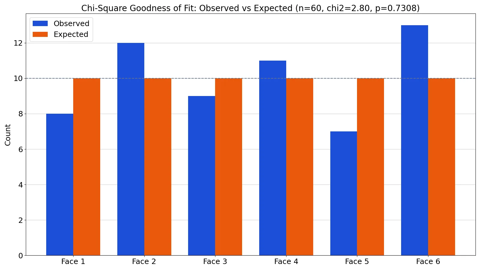
A die-roll experiment recorded 60 rolls and compared the observed counts per face to a uniform expectation of 10 per face.

Face	Observed	Expected
1	8	10
2	12	10
3	9	10
4	11	10
5	7	10
6	13	10

The total is $n = 60$, and the expected count per face is $E = n/6 = 60/6 = 10.0000$.

Now apply the formula $\chi^2 = \sum (O - E)^2 / E$ term by term.

Face 1: $(8 - 10.0000)^2 / 10.0000 = 0.4000$
Face 2: $(12 - 10.0000)^2 / 10.0000 = 0.4000$
Face 3: $(9 - 10.0000)^2 / 10.0000 = 0.1000$
Face 4: $(11 - 10.0000)^2 / 10.0000 = 0.1000$
Face 5: $(7 - 10.0000)^2 / 10.0000 = 0.9000$
Face 6: $(13 - 10.0000)^2 / 10.0000 = 0.9000$

Summing those six terms gives $\chi^2 = 2.8000$.

The degrees of freedom are $df = k - 1 = 6 - 1 = 5$. The p-value is $p = P(\chi^2_5 > 2.8000) = 0.7308$. The critical value at $\alpha = 0.05$ is $\chi^2_{crit} = 11.0705$.

Since $p = 0.7308 \ge 0.05$, you fail to reject $H_0$. The observed counts are consistent with a fair die.

Here is the same test in Python:

from scipy import stats
observed = [8, 12, 9, 11, 7, 13]
expected = [10.0000]*6
chi2, p = stats.chisquare(observed, expected)
print(f"chi2 = {chi2:.4f}, df = {len(observed) - 1}, p = {p:.4f}")

Output:

chi2 = 2.8000, df = 5, p = 0.7308

Other Ways to Do It

Spreadsheets handle this test with two columns and one formula. Put observed counts in one column and expected counts in another, then compute each term with a formula like =(A2-B2)^2/B2 and sum the column. The p-value comes from =CHISQ.DIST.RT(chi2, df) in Excel, where the first argument is your statistic and the second is the degrees of freedom.

Statistical software packages automate the whole procedure. Many commercial packages choose bin endpoints so that group membership is equiprobable, which tends to maximize power [2]. The chi-square goodness of fit test works for any univariate distribution, which makes it more flexible than the Kolmogorov-Smirnov and Anderson-Darling tests, since those are restricted to continuous distributions [1].

If your question is about a mean rather than a distribution, a different test applies. The T-Test Calculator covers that case.

Troubleshooting

Expected counts below 5. Combine adjacent categories with small expectations, or increase your sample size. The rule of thumb exists because the chi-square approximation degrades when expected counts are tiny [2].

Degrees of freedom look wrong. Count your categories carefully. If you estimated a parameter such as a rate or a shape parameter from the same data, subtract one additional degree of freedom per estimated parameter.

Probabilities do not sum to 1. Check your null hypothesis. Expected counts must sum to the sample size, and null probabilities must sum to 1.

Statistic is huge. A very large statistic lands far out in the right tail and produces a very small p-value [3]. That is evidence against the null, but check for data entry errors before you interpret it.

Continuous data with no natural bins. You must create intervals yourself. The choice of endpoints changes the statistic, so report how you binned the data [1].

Common Mistakes

Using raw measurements instead of counts. The test operates on binned data, so build a frequency table first [1]. Fix: convert your data to counts per category before computing anything.
Ignoring the expected count rule. Categories with expected counts far below 5 distort the p-value. Fix: merge sparse categories or gather more observations.
Forgetting to subtract estimated parameters from df. If you fit parameters from the data, $df = k - 1 - m$ where $m$ is the number of estimated parameters. Fix: count every parameter you estimated.
Treating a large p-value as proof of the null. Failing to reject means the data are consistent with the claimed distribution, not that the distribution is correct. Fix: describe the result as "no evidence against" the null.
Reusing the same data to pick bins and test the hypothesis. The statistic depends on the binning, so data-driven bins inflate the apparent fit [1]. Fix: define bins before looking at the counts, or use equiprobable bins chosen from the null distribution [2].
Applying the test to dependent observations. Repeated measurements on the same subject violate independence. Fix: aggregate to one count per independent unit.

Limitations

The chi-square goodness of fit test tells you whether the counts differ from expectation overall. It does not tell you which category is responsible, and it does not measure the size of the departure. A small p-value says "something differs" without saying how much or where. Follow up with per-category contributions $(O - E)^2 / E$ to see which cells drive the statistic.

The test is also sensitive to sample size and binning choices. With a very large sample, trivial departures from the null can produce small p-values. With a small sample, real departures can go undetected. The number of groups and how group membership is defined affect the power of the test, and only useful rules of thumb exist for choosing them [2]. Treat the result as one piece of evidence, not a verdict.

Frequently Asked Questions

What are the requirements to perform a goodness of fit test?

You need count data in mutually exclusive categories, independent observations, a fully specified null distribution with probabilities summing to 1, and expected counts of at least 5 per category as a rule of thumb [2]. You also need a large enough sample for the chi-square approximation to be reasonable [1].

Can I use a goodness of fit test with continuous data?

Yes, but you must bin the data into non-overlapping intervals first [2]. The test statistic depends on how you bin, so choose intervals before examining the counts, or use equiprobable intervals based on the null distribution [2][1].

What happens if my expected counts are less than 5?

The chi-square approximation becomes unreliable. Combine categories with small expected counts into larger ones, or collect more data. The at-least-5 rule is a rule of thumb rather than a hard law, but it is widely used [2].

How do I calculate the degrees of freedom?

For a simple null hypothesis with no estimated parameters, $df = k - 1$, where $k$ is the number of categories. If you estimated $m$ parameters from the data, use $df = k - 1 - m$.

What does a large p-value mean here?

It means the observed counts are close enough to the expected counts that chance alone could explain the differences. In the die example, $p = 0.7308$ means you fail to reject the null. It does not prove the die is fair, only that this sample gives no evidence against fairness.