Excel INDEX MATCH: How to Look Up Values Step by Step

By Dr. Zubair Khalid, DVM, MS, PhD · 2026-10-03

Excel INDEX MATCH is a lookup technique that combines two functions: MATCH finds the position of a value in a column, and INDEX returns the value at that position in another column. Together they look up a value in a table without the leftmost-column restriction that VLOOKUP has. This guide shows the syntax, a worked example, and the fixes for common errors.

Quick Answer

MATCH returns the relative position of a lookup value inside a range, for example =MATCH(25,A1:A3,0) returns 2 because 25 is the second item [1].
INDEX returns a value or reference from a table or range, selected by row and column number [2].
The combined pattern is =INDEX(return_range, MATCH(lookup_value, lookup_range, 0)).
The 0 in MATCH forces an exact match, which is what you want for IDs, names, and codes.
INDEX MATCH can look left as well as right, and it can calculate faster than VLOOKUP on large datasets [3].

Before You Start

You need two things in place before you write the formula.

First, a lookup column that contains the value you are searching for, such as a product ID. Second, a return column that contains the value you want back, such as a price. The two columns do not have to sit next to each other, and the return column can be to the left of the lookup column. That flexibility is the main reason people switch from VLOOKUP.

You also need to decide on the match type. The MATCH function takes a match_type argument of -1, 0, or 1, and the default is 1 [1]. For lookups of IDs, names, and codes, always use 0 for an exact match. If you leave the argument out, MATCH assumes an approximate match and expects sorted data, which produces wrong answers on unsorted tables.

One more habit worth building: keep the lookup range and the return range the same height. If MATCH searches A2:A6 and INDEX reads C2:C6, both ranges cover five rows, so the position MATCH returns lines up with the row INDEX reads.

Step by Step

Identify the lookup value. This is the cell holding what you want to find, such as a product ID in D2.
Identify the lookup range. This is the column where that value lives, such as the Product ID column A2:A6.
Identify the return range. This is the column holding the answer, such as the Price column C2:C6.
Write MATCH first. =MATCH(D2,A2:A6,0) returns the position of the ID inside the range. If D2 holds P003, MATCH returns 3 because P003 is the third item in A2:A6 [1].
Wrap INDEX around it. =INDEX(C2:C6,MATCH(D2,A2:A6,0)) uses that position as the row number and returns the third value in C2:C6 [2].
Press Enter and check the result. The formula should return the price that belongs to the ID in D2.
Copy the formula down. Lock the ranges first, as in =INDEX($C$2:$C$6,MATCH(D2,$A$2:$A$6,0)), then drag the fill handle or copy the cell to the rows below. Only the relative lookup cell shifts, so each row looks up its own ID.

The general form is:

$$=\text{INDEX}(\text{return\_range},\ \text{MATCH}(\text{lookup\_value},\ \text{lookup\_range},\ 0))$$

If you need to match on both a row and a column, the pattern extends to INDEX MATCH MATCH, which uses two MATCH functions to supply both the row number and the column number. That approach is covered in Excel INDEX MATCH with Multiple Criteria: Step by Step.

Worked Example

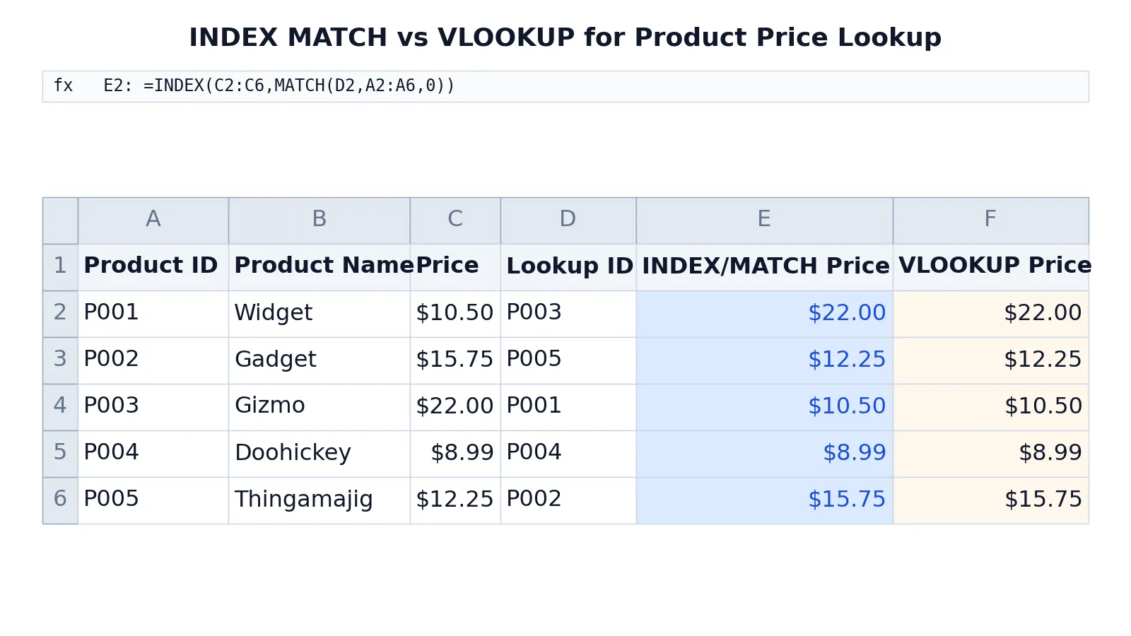
The table below is a small product list. Column A holds product IDs, column B holds product names, and column C holds prices. Column D holds the IDs you want to look up, column E returns the price with INDEX MATCH, and column F returns the same price with VLOOKUP for comparison.

Row	A	B	C	D	E	F
1	Product ID	Product Name	Price	Lookup ID	INDEX/MATCH Price	VLOOKUP Price
2	P001	Widget	10.5	P003	`=INDEX(C2:C6,MATCH(D2,A2:A6,0))` -> displays $22.00	`=VLOOKUP(D2,A2:C6,3,FALSE)` -> displays $22.00
3	P002	Gadget	15.75	P005	`=INDEX(C2:C6,MATCH(D3,A2:A6,0))` -> displays $12.25	`=VLOOKUP(D3,A2:C6,3,FALSE)` -> displays $12.25
4	P003	Gizmo	22	P001	`=INDEX(C2:C6,MATCH(D4,A2:A6,0))` -> displays $10.50	`=VLOOKUP(D4,A2:C6,3,FALSE)` -> displays $10.50
5	P004	Doohickey	8.99	P004	`=INDEX(C2:C6,MATCH(D5,A2:A6,0))` -> displays $8.99	`=VLOOKUP(D5,A2:C6,3,FALSE)` -> displays $8.99
6	P005	Thingamajig	12.25	P002	`=INDEX(C2:C6,MATCH(D6,A2:A6,0))` -> displays $15.75	`=VLOOKUP(D6,A2:C6,3,FALSE)` -> displays $15.75

Take cell E2. The lookup ID in D2 is P003. MATCH searches A2:A6 for P003 and finds it in the third position. INDEX then reads the third value in C2:C6, which is 22, and the cell displays $22.00. The VLOOKUP in F2 reaches the same answer, but only because the lookup column happens to be the leftmost column of its range.

The two formulas agree on every row here. The difference shows up when your return column sits to the left of your lookup column, or when you insert a column in the middle of the table. VLOOKUP breaks in both cases because it counts columns from the left edge of its range. INDEX MATCH does not care about column order.

Other Ways to Do It

VLOOKUP is the older option. It searches the first column of a range and returns a value from a column you count off to the right. It works well when your data is already arranged that way, and it is easier to read at a glance. The trade-off is the leftmost-column rule and the fragile column index number.

XLOOKUP is the modern replacement in Excel for Microsoft 365, Excel 2024, and Excel 2021 [4]. It takes a lookup range and a return range directly, defaults to an exact match, and handles the left-lookup case natively. If your version has it, XLOOKUP is usually the shortest formula.

XMATCH is the newer version of MATCH. It searches in any direction and returns exact matches by default [1][5]. You can pair it with INDEX the same way, as in =INDEX(C6:E12,XMATCH(B3,B6:B12),XMATCH(C3,C5:E5)) for a two-way lookup [5].

INDEX MATCH MATCH extends the pattern to two dimensions. One MATCH supplies the row, the other supplies the column, and INDEX returns the intersection.

If you are still deciding between these options, Excel Lookup Functions: VLOOKUP, XLOOKUP and INDEX-MATCH compares them side by side. For the MATCH function on its own, see Excel MATCH Function: Syntax and Examples.

Troubleshooting

#N/A error. MATCH returns #N/A when it cannot find the lookup value in the lookup array [6]. Check for trailing spaces and numbers stored as text. Case differences do not cause #N/A because MATCH is not case-sensitive. A quick test is to compare the two cells with =A2=D2, which returns FALSE when a space or a text-versus-number mismatch separates them (it ignores case, so use =EXACT(A2,D2) to compare case too).

#VALUE! error. This often appears when INDEX is used as an array formula with MATCH and the formula was not entered as an array formula [4]. In Excel for Microsoft 365, dynamic arrays handle most of these cases automatically.

Wrong but valid result. If MATCH returns a position that looks off, check the third argument. A missing or nonzero match_type triggers approximate matching, which needs sorted data and can return the wrong row [6].

Formula breaks after inserting a column. This is the classic VLOOKUP failure. INDEX MATCH survives column inserts because it references ranges, not column counts.

Result shifts when you copy down. Check that your ranges use the right mix of absolute and relative references. Locking the ranges with dollar signs keeps them fixed while the lookup cell moves.

Common Mistakes

Leaving out the 0 in MATCH. Without it, MATCH defaults to approximate matching and expects ascending order [1]. Fix: always type the third argument as 0 for exact lookups.
Mismatched range sizes. If MATCH searches A2:A6 but INDEX reads C2:C10, the positions no longer line up. Fix: make both ranges cover the same number of rows.
Mixing text and numbers. An ID stored as text will not match the same ID stored as a number. Fix: convert one side so both are the same type, or use a formula that coerces the type.
Forgetting to lock the ranges. Copying a formula down without absolute references shifts the lookup range row by row. Fix: use $A$2:$A$6 and $C$2:$C$6.
Hiding errors with IFERROR too early. Wrapping the formula in IFERROR before it works correctly hides the real problem [6]. Fix: get the formula returning correct values first, then add error handling.
Assuming INDEX MATCH is always faster. The speed advantage depends on the scenario, and it is not guaranteed in every workbook [3]. Fix: test on your own data if performance matters.

Limitations

INDEX MATCH returns the first match it finds. If your lookup column contains duplicate IDs, you get the value for the first one and no warning that others exist. To review duplicates before you build lookups, see How to Find Duplicates in Excel (Step by Step).

The technique also does not clean your data. Trailing spaces and mixed data types cause #N/A errors that look like formula problems but are really data problems. And while INDEX MATCH can be faster than VLOOKUP on large datasets, the gain varies by scenario and is not something to count on without testing [3]. For very large or frequently refreshed tables, a different structure may serve you better.

Frequently Asked Questions

Why is INDEX MATCH better than VLOOKUP?

INDEX MATCH can return a value from a column to the left of the lookup column, and it does not break when you insert or delete columns inside the table. VLOOKUP counts columns from the left edge of its range, so any structural change shifts its column index. INDEX MATCH also has evidence of calculating faster than VLOOKUP in some scenarios [3].

What does the 0 mean in MATCH?

The 0 is the match_type argument, and it tells MATCH to find an exact match [1]. Without it, MATCH defaults to 1, which finds the largest value less than or equal to the lookup value and requires the data to be sorted ascending. For IDs and names, always use 0.

Can INDEX MATCH look up values to the left?

Yes. INDEX reads from whatever range you give it, and MATCH searches a separate range. Neither function requires the return column to sit to the right of the lookup column. That is the main structural advantage over VLOOKUP.

How do I fix a #N/A error in INDEX MATCH?

Start by confirming the lookup value exists in the lookup range. MATCH returns #N/A when it finds nothing [6]. Then check for trailing spaces, text-versus-number mismatches, and a missing 0 in the match type. Only add IFERROR after the formula returns correct values on its own.

Can I use INDEX MATCH with more than one condition?

Yes. You can combine conditions inside the MATCH lookup array, or use two MATCH functions to supply both a row and a column. The two-way version is often written as INDEX MATCH MATCH. For a full walkthrough, see Excel INDEX MATCH with Multiple Criteria: Step by Step.

Once the basic pattern is in place, you can reuse it across most lookup tasks in a workbook. If you want to see where lookups fit into a wider workflow, How to Analyse Data in Excel: Step by Step covers the surrounding steps.