Does Not Equal in Excel: The <> Operator Explained

By Dr. Zubair Khalid, DVM, MS, PhD · 2026-10-03

Does not equal in Excel is written with the operator <>. You place it between two values or expressions, and Excel returns TRUE when they differ and FALSE when they match. The same operator works inside IF tests and inside COUNTIF criteria, which is where most people first need it.

Quick Answer

The operator is <>, a less-than sign followed by a greater-than sign, with no space between them [1].
=A2<>"Widget" returns TRUE when A2 is anything other than the exact text Widget, and FALSE when it matches.
Comparison operators like <> are one of the four operator types in Excel, alongside arithmetic, text concatenation, and reference operators [1].
In COUNTIF and similar criteria, you write the operator inside the quoted text, as in "<>Widget".
<> is not case-sensitive for text, so "widget" and "Widget" compare as equal.

Before You Start

You need to know three things before writing a not-equal formula.

First, <> is a comparison operator, not an arithmetic one. It does not calculate a number. It produces a logical value, TRUE or FALSE, which you then feed into IF, COUNTIF, conditional formatting, or another function [2].

Second, the two sides of the comparison must be the same kind of thing. Comparing a number to text gives a result you probably did not intend, because Excel ranks data types in a fixed order when it compares them.

Third, text comparisons ignore case. "Widget" and "widget" are treated as equal, so =A2<>"widget" returns FALSE when A2 contains Widget. If you need a case-sensitive not-equal test, <> alone will not do it.

One more detail matters for criteria. When you type a criterion into COUNTIF, SUMIF, or a similar function, the whole criterion goes inside double quotes, including the operator. So the formula reads "<>Widget", not <>"Widget".

Step by Step

Pick the two things to compare. They can be two cells, a cell and a literal value, or two expressions. For example, A2 and the text "Widget".

Put <> between them. The formula =A2<>"Widget" compares the two. Excel returns TRUE if they differ and FALSE if they are the same.

Wrap it in IF if you want words instead of TRUE/FALSE. The IF function takes a logical test and returns one value when the test is TRUE and another when it is FALSE [3]. So =IF(A2<>"Widget","Not a widget","Widget") gives you readable output.

For counting, move the operator inside the quotes. In COUNTIF, the criterion "<>Widget" counts every cell in the range that is not exactly Widget. The operator and the value both live inside one pair of double quotes.

Check the result against a small range first. Build the formula on a handful of rows where you already know the answer, then extend it to the full dataset.

If you want to combine a not-equal test with other conditions, the NOT function is the alternative route. NOT reverses the value of its argument, so NOT(A2="Widget") gives the same result as A2<>"Widget" [4]. Both are valid. The <> form is shorter and is what most people use.

Worked Example

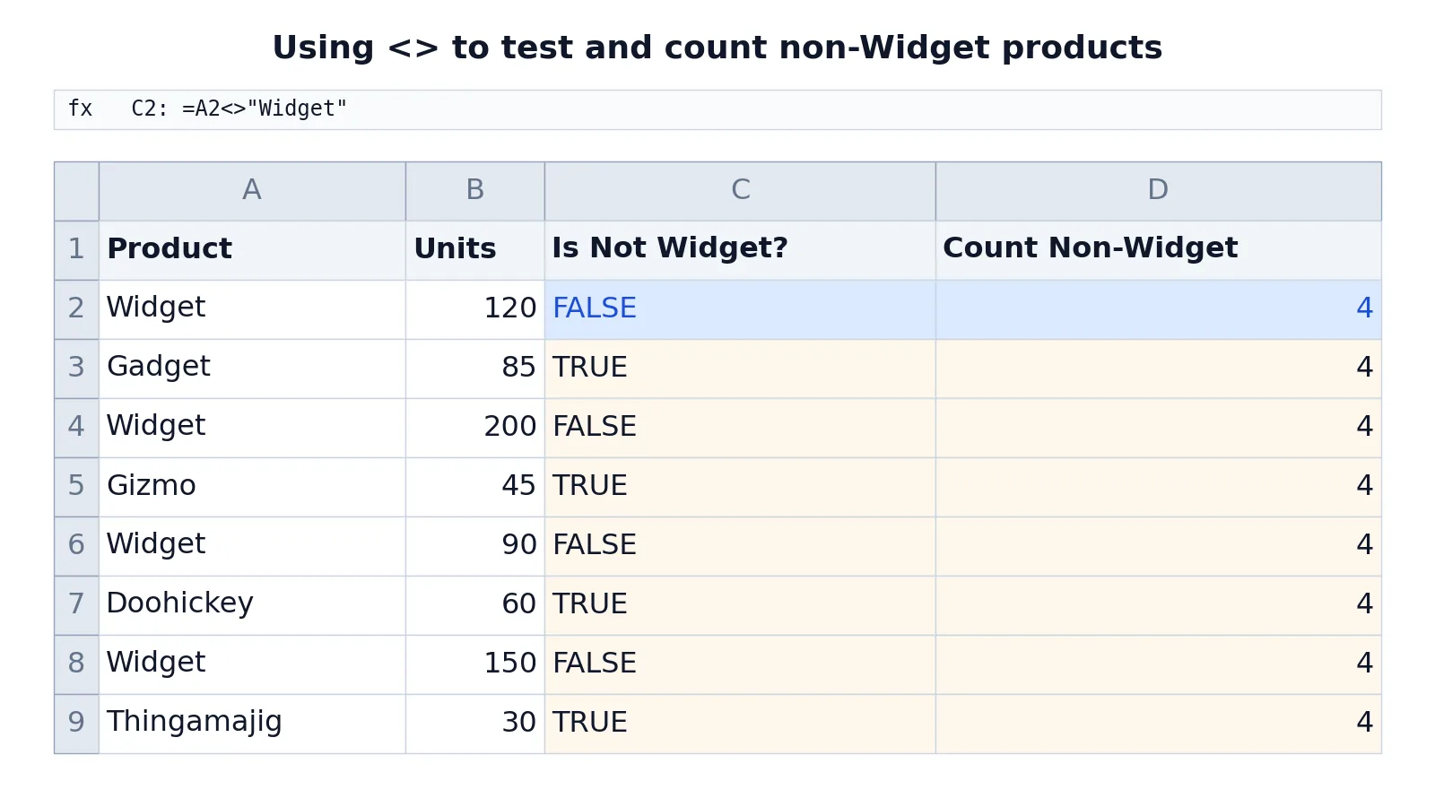
This sheet lists eight products with their unit counts. Column C tests each product name against the text Widget, and cell D2 counts how many products are not Widget.

	A	B	C	D
1	Product	Units	Is Not Widget?	Count Non-Widget
2	Widget	120	`=A2<>"Widget"` -> FALSE	`=COUNTIF($A$2:$A$9,"<>Widget")` -> 4
3	Gadget	85	`=A3<>"Widget"` -> TRUE	`=COUNTIF($A$2:$A$9,"<>Widget")` -> 4
4	Widget	200	`=A4<>"Widget"` -> FALSE	`=COUNTIF($A$2:$A$9,"<>Widget")` -> 4
5	Gizmo	45	`=A5<>"Widget"` -> TRUE	`=COUNTIF($A$2:$A$9,"<>Widget")` -> 4
6	Widget	90	`=A6<>"Widget"` -> FALSE	`=COUNTIF($A$2:$A$9,"<>Widget")` -> 4
7	Doohickey	60	`=A7<>"Widget"` -> TRUE	`=COUNTIF($A$2:$A$9,"<>Widget")` -> 4
8	Widget	150	`=A8<>"Widget"` -> FALSE	`=COUNTIF($A$2:$A$9,"<>Widget")` -> 4
9	Thingamajig	30	`=A9<>"Widget"` -> TRUE	`=COUNTIF($A$2:$A$9,"<>Widget")` -> 4

Column C returns FALSE on rows 2, 4, 6, and 8 because those cells contain Widget. It returns TRUE on rows 3, 5, 7, and 9 because Gadget, Gizmo, Doohickey, and Thingamajig all differ from Widget.

Cell D2 counts the same thing across the whole range. Four of the eight products are not Widget, so COUNTIF returns 4. The dollar signs in $A$2:$A$9 lock the range so the formula can be copied without shifting.

Notice the two different placements of the operator. In column C, <> sits between two operands as a normal comparison. In D2, <> sits inside the quoted criterion string. Mixing these up is the most common source of errors with this operator.

Other Ways to Do It

NOT with equals. =NOT(A2="Widget") produces the same TRUE/FALSE result as =A2<>"Widget" [4]. Use this when you are already building a compound test with AND or OR, since NOT reads naturally inside those functions [5].

IF with a not-equal test. =IF(A2<>"Widget","Keep","Skip") turns the logical result into labels. The IF function returns the first value when the test is TRUE and the second when it is FALSE [3].

COUNTIFS for multiple conditions. When you need more than one criterion, COUNTIFS accepts several range and criterion pairs. One of them can carry the <> operator.

Conditional formatting. A formula rule such as =A2<>"Widget" highlights every cell that is not Widget. You enter it through Conditional Formatting and the "Use a formula to determine which cells to format" option [5].

SUMIF with a not-equal criterion. =SUMIF($A$2:$A$9,"<>Widget",$B$2:$B$9) adds the Units values for every row whose product is not Widget. The criterion syntax is identical to COUNTIF.

If you are comparing numbers instead of text, the same operator applies. =B2<>120 is TRUE whenever B2 holds anything other than 120. For related comparison work, see greater than or equal to in Excel and the Boolean formula guide.

Troubleshooting

The formula returns TRUE when you expected FALSE. Check for trailing spaces. "Widget " with a space at the end is not equal to "Widget", so the test returns TRUE. TRIM the source data or the comparison value.

COUNTIF returns a number that looks too high. Blank cells in the range count as not equal to your criterion. If your range extends past the data, "<>Widget" will count every empty cell below the last row.

The criterion returns 0 when it should not. You may have written <>"Widget" inside the quotes, producing "<>"Widget"". The operator and the value belong inside one pair of quotes: "<>Widget".

Text and numbers compare oddly. Excel orders data types when comparing across them, so a number is never equal to text that looks like the same number. Convert one side so both are the same type.

Case differences are ignored. <> treats Widget and widget as equal. If case matters, you need a different approach, such as comparing with the EXACT function.

Common Mistakes

Putting quotes around the wrong part. In a plain formula, the text value gets quotes and the operator does not: =A2<>"Widget". In a COUNTIF criterion, both go inside one pair of quotes: "<>Widget". Fix by matching the pattern to the context.
Writing =<> or ><. The operator is exactly two characters in the order less-than then greater-than. Reversed or split, Excel rejects the formula.
Forgetting that blanks count as not equal. An empty cell is not equal to any text value, so it passes a <> test. Restrict the range to the actual data.
Assuming case sensitivity. <> ignores case for text. Use EXACT when case matters.
Comparing text to numbers. "120" and 120 are different types and will not compare as equal. Keep both sides consistent.
Copying a COUNTIF range without locking it. Use absolute references like $A$2:$A$9 so the range does not drift when you fill the formula down.

Limitations

The <> operator cannot express "not equal to any of these values" on its own. A single comparison handles one value at a time. To exclude several values you need COUNTIFS with multiple criteria, or a different construction entirely.

It also cannot distinguish case, and it cannot see through formatting. A cell that displays Widget but stores "Widget " with a trailing space is not equal to Widget, and the formula will tell you so even though the sheet looks correct. Cleaning source data before you compare is usually faster than debugging the formula afterward.

Frequently Asked Questions

How do you type does not equal in Excel?

Type a less-than sign immediately followed by a greater-than sign, with no space between them. On a standard keyboard that is Shift+comma then Shift+period. The result is <>, which Excel reads as a comparison operator [1].

Why does my COUNTIF with <> return the wrong count?

The most common cause is a range that includes blank cells, since blanks are not equal to your criterion and get counted. The second most common cause is misplaced quotes. The criterion must be one quoted string such as "<>Widget", with the operator inside the quotes.

Is <> the same as the NOT function?

They produce the same logical result in a simple test. =A2<>"Widget" and =NOT(A2="Widget") both return TRUE when A2 is not Widget [4]. The operator is shorter, while NOT is easier to read inside AND and OR combinations [5].

Does <> work with numbers and dates?

Yes. =B2<>120 returns TRUE when B2 holds any value other than 120, and the same pattern works for dates. The comparison follows the same rules regardless of the data type, as long as both sides are the same type.

Can I use <> in conditional formatting?

Yes. A formula rule such as =A2<>"Widget" formats every cell that is not Widget. You create it from Conditional Formatting by choosing the option to use a formula to determine which cells to format [5]. For more logical building blocks, see IF AND statements in Excel and the Excel IS functions.