What Is Descriptive Statistics? Definition and Examples

By Dr. Zubair Khalid, DVM, MS, PhD · 2026-10-03

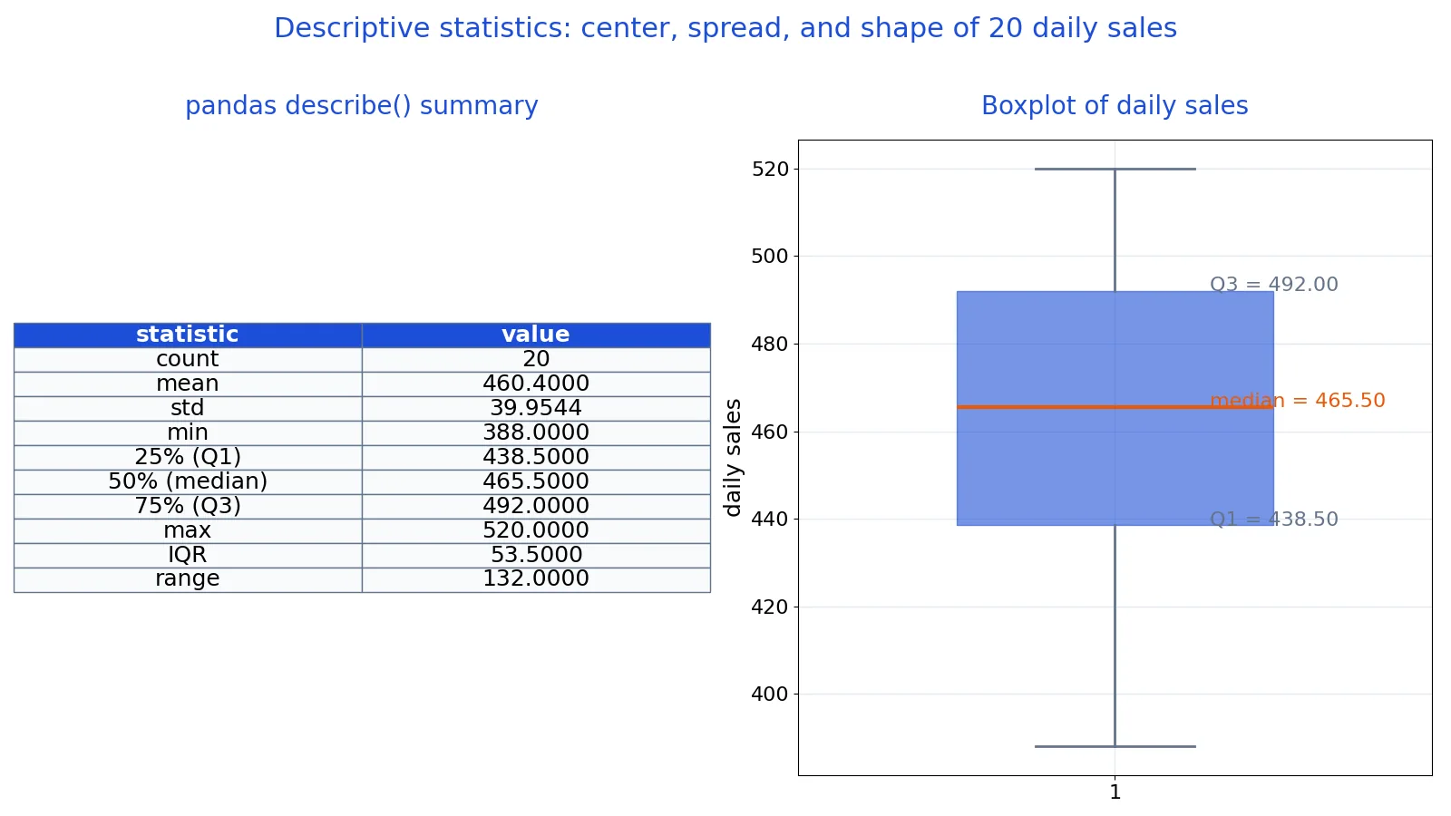
A descriptive statistic is a number that summarizes a dataset without drawing conclusions beyond it. The mean, median, standard deviation, and range are all descriptive statistics, and together they tell you where your data sits, how spread out it is, and what shape it takes. This article defines the term, explains the main measures, and walks through a full example.

Quick Answer

A descriptive statistic summarizes observed data. It describes what you measured, not what you can infer about a larger group.
Measures of center (mean, median, mode) answer "where is the middle of the data?"
Measures of spread (range, variance, standard deviation, interquartile range) answer "how far apart are the values?"
Measures of shape (skewness, kurtosis) and graphs (histograms, boxplots) answer "what does the distribution look like?"
Descriptive statistics are the starting point of any analysis. They help you spot outliers, missing values, and unusual patterns before you run formal tests [1].

What Descriptive Statistics Means

In plain terms, descriptive statistics is the branch of statistics that organizes, displays, and summarizes a collection of data [2]. You use it whenever you report a count, an average, or a chart.

The precise definition is narrower. Descriptive statistics is the set of numerical and graphical methods that summarize the characteristics of a sample or population without using probability to generalize beyond the observed data [3]. Every value you compute describes the data in front of you.

This separates descriptive work from inferential work. Inferential statistics uses sample data to estimate population values and to test hypotheses. Descriptive statistics stops at the summary. If you want the contrast in detail, see descriptive vs inferential statistics.

Descriptive methods cover three families of measures:

Family	Question it answers	Common measures
Center	Where is the middle?	Mean, median, mode
Spread	How variable is the data?	Range, variance, standard deviation, IQR
Shape	What does the distribution look like?	Skewness, kurtosis, histogram, boxplot

How It Works

Each measure reduces a list of values to a single number using a formula. The most common ones are below.

Mean. The arithmetic average.

$$\bar{x} = \frac{\sum_{i=1}^{n} x_i}{n}$$

Here $\bar{x}$ is the sample mean, $x_i$ is each individual value, $n$ is the number of values, and $\sum$ means "add them all up." The mean uses every value, so extreme values pull it.

Median. Sort the values from smallest to largest. The median is the middle value. With an even count, it is the average of the two middle values. The median ignores how far the extremes sit, so it resists outliers.

Variance and standard deviation. Variance measures the average squared distance from the mean. The sample standard deviation is its square root, which returns the units to the original scale.

$$s = \sqrt{\frac{\sum_{i=1}^{n}(x_i - \bar{x})^2}{n-1}}$$

Here $s$ is the sample standard deviation, $x_i - \bar{x}$ is each value's deviation from the mean, and $n-1$ is the degrees of freedom used for a sample. Software such as SciPy's describe function reports the unbiased variance with denominator $n-1$ by default [4].

Quartiles and IQR. Q1 is the value below which 25% of the data falls. Q3 is the 75% mark. The interquartile range is $IQR = Q3 - Q1$, and it covers the middle half of the data.

Range. The maximum minus the minimum. It is the simplest spread measure and the most sensitive to a single extreme value.

Worked Example

The dataset is 20 daily sales figures in dollars for a small retail shop.

Day	Sales	Day	Sales
1	412	11	431
2	388	12	489
3	455	13	455
4	501	14	512
5	476	15	478
6	399	16	396
7	520	17	463
8	445	18	507
9	468	19	441
10	502	20	470

Step 1: Count and sum. There are $n = 20$ values. Their sum is 9208.

Step 2: Mean. $9208 / 20 = 460.4000$. The shop averaged $460.40 in daily sales.

Step 3: Sort the values.

388, 396, 399, 412, 431, 441, 445, 455, 455, 463, 468, 470, 476, 478, 489, 501, 502, 507, 512, 520

Step 4: Median. With 20 values, the middle two are the 10th and 11th: 463 and 468. The median is $(463 + 468) / 2 = 465.5000$.

Step 5: Quartiles. Using linear interpolation, Q1 = 438.5000 and Q3 = 492.0000.

Step 6: IQR. $492.0000 - 438.5000 = 53.5000$.

Step 7: Range. $520.0 - 388.0 = 132.0000$.

Step 8: Standard deviation. The sample standard deviation is 39.9544. A spreadsheet check with STDEV.S returns the same value.

You can reproduce all of this in one call:

import pandas as pd
sales = [412, 388, 455, 501, 476, 399, 520, 445, 468, 502,
         431, 489, 455, 512, 478, 396, 463, 507, 441, 470]
s = pd.Series(sales)
print(s.describe())

Output:

count    20.000000
mean     460.400000
std      39.954448
min      388.000000
25%      438.500000
50%      465.500000
75%      492.000000
max      520.000000

The describe() method returns a compact descriptive summary in one step [5]. The mean (460.40) sits slightly below the median (465.50), which hints at mild left skew from the low values of 388 and 396.

How to Interpret It

Read the center and spread together. A mean of 460.40 with a standard deviation of 39.95 means a typical day lands roughly $40 away from the average. The range of 132 shows the full swing between the best and worst days.

Compare the mean and median. When they are close, the distribution is roughly symmetric. When the mean is pulled below or above the median, extreme values are at work. Here the gap is small, so no single day dominates the picture.

Use the IQR to judge what counts as unusual. A common rule flags values below $Q1 - 1.5 \times IQR$ or above $Q3 + 1.5 \times IQR$. For this data, that is below 358.25 or above 572.25. No day crosses either line, so there are no outliers by that rule.

Graphs often reveal what numbers hide. A histogram shows where values cluster, and a boxplot shows the quartiles and any points outside the whiskers [3]. The boxplot for this dataset spans 388.0 to 520.0 with a box from 438.50 to 492.00.

When to Use It (and when not to)

Use descriptive statistics at the start of every analysis. They help you check data quality, spot missing values and outliers, and choose appropriate methods later [1]. They are also the right tool when your goal is simply to report what happened, such as summarizing survey responses, test scores, or sales figures.

Use them when you have a full census of the group you care about. If you measured every member, the summary is the answer, and no inference is needed. The census definition covers that case.

Do not use descriptive statistics alone to claim that a difference between groups is real. A higher mean in one group does not prove the groups differ in the population. That claim needs inferential methods such as confidence intervals or hypothesis tests.

Do not use them to predict future values. A mean of 460.40 describes the past 20 days. It says nothing about tomorrow.

Descriptive Statistics vs Inferential Statistics

The two branches answer different questions. Descriptive statistics summarizes the data you have. Inferential statistics uses that data to make statements about a larger group, with a stated level of uncertainty.

Aspect	Descriptive statistics	Inferential statistics
Goal	Summarize observed data	Generalize to a population
Typical tools	Mean, median, SD, charts	Confidence intervals, t-tests, regression
Uses probability	No	Yes
Example question	What was the average daily sale?	Is the average sale higher this year?
Output	Numbers and graphs	Estimates, p-values, intervals

A single dataset can support both. You compute descriptive statistics first, then use them as inputs to inference.

Common Mistakes

Reporting the mean for skewed data. The mean gets dragged by extreme values. Check the median too, and report it when the distribution is skewed.
Confusing the standard deviation with the standard error. The standard deviation describes spread in your data. The standard error describes uncertainty in an estimate. They are different quantities.
Using the population formula for a sample. Dividing by $n$ instead of $n-1$ underestimates the variance. Match the formula to whether you have a sample or a full population.
Ignoring the units. A standard deviation of 39.95 is meaningless without knowing it is dollars. Always attach units to center and spread measures.
Treating a summary as the whole story. Two datasets can share a mean and standard deviation and look completely different. Plot the data.
Dropping missing values silently. A count of 20 when you started with 25 rows hides five missing entries. Report how missing values were handled [1].

Limitations

Descriptive statistics cannot tell you whether a pattern is statistically significant or whether it generalizes beyond your data. A summary also compresses information, and compression loses detail. The mean and standard deviation alone cannot distinguish a symmetric distribution from a bimodal one with the same values.

The measures are also sensitive to how the data was collected. A biased sample produces a biased summary, and no formula fixes that. Outliers and measurement errors distort the mean, range, and standard deviation more than the median and IQR, so the choice of measure matters. Always pair the numbers with a graph and a note on how the data was gathered.

Frequently Asked Questions

What is a descriptive statistic in simple terms?

It is a single number that sums up a set of data. The average of your test scores, the range of your daily step counts, and the middle value of your commute times are all descriptive statistics. They describe the data you collected.

What are the three main types of descriptive statistics?

Measures of center, measures of spread, and measures of shape. Center covers the mean, median, and mode. Spread covers the range, variance, standard deviation, and IQR. Shape covers skewness, kurtosis, and the graphs that display the distribution.

Is the mean a descriptive statistic?

Yes. The mean is one of the most common descriptive statistics. It summarizes a list of values with a single average. It becomes part of inferential work only when you use it to estimate a population value or test a hypothesis.

What is the difference between descriptive and inferential statistics?

Descriptive statistics summarizes the data you observed. Inferential statistics uses that summary to make claims about a larger population, with a measure of uncertainty attached. Descriptive work needs no probability model. Inference does.

Can descriptive statistics prove a hypothesis?

No. Descriptive statistics can show a pattern in your data, such as one group having a higher average. Proving that the pattern is real in the population requires a hypothesis test or confidence interval. Those are inferential tools.