How to Choose a Calculator for Statistical Analysis in Research
By Dr. Zubair Khalid, DVM, MS, PhD ·

By the end of this guide you will be able to match a calculator for statistical analysis in research to your actual study design, run a complete analysis from raw numbers to a reported result, verify the output with an independent check, and avoid the mistakes that most often invalidate student projects and first manuscripts. To follow the worked examples, have a laptop with R and RStudio installed (both are free) or Python 3 with the SciPy library, plus any spreadsheet program. Every example below runs on a dozen numbers you can type by hand.
The phrase covers more ground than most newcomers expect. In a research setting, a statistical calculator is any tool that turns raw data into descriptive statistics, test statistics, p-values, and confidence intervals. That includes a handheld scientific calculator, a web page with a t-test box, a spreadsheet, a point-and-click package such as SPSS or GraphPad Prism, a scripted language such as R or Python, and dedicated suites for specific designs such as meta-analysis software. Choosing well is a design decision, not a shopping decision.
What a "Calculator" Means in Modern Research
Two layers of vocabulary make the choice easier. Descriptive statistics summarize the data you collected, for example a mean, a standard deviation, or a percentage. Inferential statistics use those summaries to judge whether the pattern is surprising under a null hypothesis, which is the working assumption of no effect or no association. The core outputs are three numbers. A test statistic measures how far the data fall from the null expectation. A p-value gives the probability of a result at least this extreme if the null hypothesis were true. A confidence interval gives a range of plausible values for the true effect, conventionally at the 95 percent level.
Tools differ in how much control they give you over those numbers. A handheld calculator exposes every intermediate step but offers only a handful of tests. A scripted language offers thousands of tests and full automation, hides nothing, and forgives nothing. Everything in between trades control for convenience.
The choice matters because the tool shapes the analysis. A spreadsheet makes a quick chi-square effortless and a multivariable model nearly impossible, so spreadsheet users drift toward simple tests whether or not the design calls for them. A scripted language makes automation effortless, so scripted users drift toward simulations and resampling. Neither drift is wrong, but you should choose the drift on purpose.
Choosing a Calculator for Statistical Analysis in Research: Match the Tool to the Question
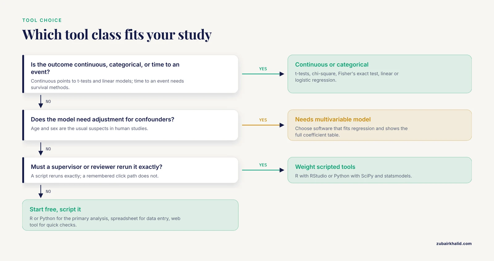
Answer four questions before you look at any product page. What type of outcome are you analyzing? How complex is the model? Who must be able to reproduce the result, and how? What can you spend in money and learning time?
The table below compares the main tool classes on those dimensions.
| Tool class | Typical examples | Best for | Cost | Reproducibility | Main risk |
|---|---|---|---|---|---|
| Handheld scientific or graphing calculator | TI-84 family, Casio fx scientific models | Coursework, exams, quick descriptive statistics | One-time purchase | None beyond your notes | Transcription errors, few tests |
| Online statistical calculator | t-test, chi-square, and sample size web tools | One-off checks and rough power estimates | Free | None unless you save the inputs | Undocumented methods, data privacy |
| Spreadsheet | Excel, Google Sheets | Data entry, small datasets, basic tests and charts | License or free | Weak, click paths are invisible | Silent autofill and copy errors |
| Point-and-click statistics package | SPSS, JMP, GraphPad Prism, Minitab | Standard tests through menus, publication graphics | Annual license | Moderate, saved output files | Undocumented click sequences |
| Scripted language | R with RStudio, Python with SciPy and statsmodels | Regression, survival analysis, simulation, automation | Free | Strong, the script is the audit trail | Steep first month |
| Meta-analysis suite | RevMan, the metafor package in R | Pooling effect sizes, heterogeneity, bias checks | Free | Strong | Pooling weak primary studies |
Simple comparisons
One t-test, one chi-square test, a handful of descriptive statistics. Any of the first three rows in the table will do. For coursework and exams, a graphing calculator from the TI-84 family or a Casio scientific model with a statistics mode computes means, standard deviations, and simple tests. For a quick check at the bench, a reputable web calculator is fine, as long as you can find out which method it uses and at what settings.
Regression and adjustment
Once predictors multiply, or once the outcome is a time to an event, you need software that fits regression models. Survival analysis is the classic case in biology and medicine. A secondary analysis of the MAPT trial followed 1,394 adults aged 70 and older who were not frail at baseline, and used a Cox proportional hazards model, a regression method for time-to-event outcomes, to test whether blood biomarkers and brain imaging measures predicted incident frailty, meaning new onset during follow-up, which occurred in 195 participants (14.0 percent) over five years [1]. No handheld calculator or spreadsheet fits that model. R with the survival package, SAS, Stata, and SPSS all do.
Meta-analysis
Pooling effect sizes across studies is its own discipline with its own software. A systematic review of quality-of-life outcomes after penile-preserving surgery for penile cancer computed risk differences (simple differences in event proportions between groups) and standardized mean differences (between-group differences expressed in standard deviation units, used when studies measure the same construct with different instruments) in RevMan version 5.4, the free package maintained by the Cochrane Collaboration, and analyzed dichotomous outcomes, meaning two-category outcomes such as yes or no, in Microsoft Excel version 17.0 [2]. A meta-analysis of infection prevalence among first responders demanded more from its tools, fitting random-effects models with restricted maximum likelihood estimation (a likelihood-based method for estimating the between-study variance), applying the Freeman-Tukey double-arcsine transformation (a variance-stabilizing transformation for proportions), reporting heterogeneity with I², τ², and 95 percent prediction intervals, and running meta-regression to explore sources of between-study differences [3]. Before you pick a meta-analysis calculator, list the estimators and diagnostics your protocol names, then confirm the software supports each one.
The Parameters That Should Drive the Decision
Outcome type and scale
Continuous outcomes such as mass, concentration, or enzyme activity point toward t-tests and linear models. Categorical outcomes such as genotype classes or infected versus not infected point toward chi-square tests, Fisher's exact test, and logistic regression. Time-to-event outcomes with censoring, meaning subjects whose event has not happened when the study ends, require survival methods. Sample size interacts with all of these, and the familiar rule of thumb for the chi-square approximation is that expected counts in each cell should be at least 5.
Sample size and power
Statistical power is the probability that a test detects a real effect of a given size. Plan it before you collect data, because no calculator rescues an underpowered sample after the fact. The pwr package in R computes the requirement from an effect size, here Cohen's d, which expresses a mean difference in standard deviation units.
library(pwr)
pwr.t.test(d = 0.5, power = 0.8, sig.level = 0.05)
Two-sample t test power calculation
n = 63.77
d = 0.5
sig.level = 0.05
power = 0.8
alternative = two.sided
NOTE: n is number in *each* groupDetecting a medium effect (d = 0.5) with 80 percent power needs about 64 subjects per group. Halve the effect size and the requirement roughly quadruples, which is why small pilot studies can only detect large effects.
Adjustment and confounding
A confounder is a variable associated with both the predictor and the outcome that can manufacture a spurious association. Age and sex are the usual suspects in human studies. If your question requires adjustment, choose a tool that fits multivariable models and shows the full coefficient table, not just a single p-value.
Reproducibility
Ask who must rerun the analysis. A supervisor, a reviewer, or you in two years can rerun a script exactly. Nobody can rerun a remembered click path. If the result will appear in a thesis or a journal, weight scripted tools heavily.
Data volume and format
Forty rows from a lab experiment and a million rows from a sequencing run are different jobs. Large omics datasets push you toward scripted tools that handle data column-wise, while a small experiment runs fine anywhere. Also consider what your instrument or database exports, because a tool that reads your raw files directly removes an entire layer of transcription errors.
Cost, licensing, and learning curve
R and Python cost nothing and run on any laptop. Paid packages buy menus, polished documentation, and support contracts. Handheld calculators cost tens of dollars and last a decade. Match the spend to the stakes, because a homework problem and a five-year cohort study do not need the same machinery.
Using a Calculator for Statistical Analysis in Research, Step by Step
This walkthrough carries a categorical dataset from raw counts to a verified, reportable result, then repeats the pattern for a continuous outcome. The commands use R because it is free and standard in the life sciences, but the sequence of steps is identical in any tool. The table below maps common designs to their usual tests.
| Outcome and design | Example | Typical test | R command |
|---|---|---|---|
| Continuous, two independent groups | enzyme activity, treated vs control | Welch t-test | t.test(x, y) |
| Continuous, paired | before and after on the same subjects | paired t-test | t.test(after, before, paired = TRUE) |
| Categorical counts vs an expected ratio | offspring in a 9:3:3:1 cross | chi-square goodness of fit | chisq.test(counts, p = ...) |
| Categorical, two groups in a 2x2 table | infection by exposure status | Fisher's exact test | fisher.test(matrix(...)) |
| Continuous, several predictors | a marker adjusted for age and sex | linear or logistic regression | lm() or glm() |
| Time to an event | months until onset of a condition | Cox proportional hazards | coxph(Surv(time, event) ~ x) |
Step 1: State the question and the outcome type
Write the question in one sentence. Example: do offspring counts from a dihybrid cross fit the expected 9:3:3:1 ratio? The outcome is categorical with four classes, so the test is a chi-square goodness-of-fit test.
Step 2: Prepare the data
Counts can go straight into a vector or into a plain CSV file. Keep the raw file untouched and work on a copy, because calculators do not warn you when the input file was overwritten last week.
Step 3: Run the test
counts <- c(58, 22, 19, 9)
chisq.test(counts, p = c(9/16, 3/16, 3/16, 1/16))
Expected output:
	Chi-squared test for given probabilities

data:  counts
X-squared = 1.1029, df = 3, p-value = 0.7764
X-squared is the test statistic, df is the degrees of freedom (the number of classes minus 1), and the p-value of 0.78 says these counts are entirely consistent with a 9:3:3:1 ratio.
Step 4: Verify with a second method
Compute the same statistic by hand. With 108 offspring, the expected counts are 60.75, 20.25, 20.25, and 6.75. Then:
chi-square = (58-60.75)^2/60.75 + (22-20.25)^2/20.25
           + (19-20.25)^2/20.25 + (9-6.75)^2/6.75
           = 0.124 + 0.151 + 0.077 + 0.750
           = 1.103
The hand calculation matches the software to three decimals, which confirms both the data entry and the function call. This two-minute habit catches more errors than any other single practice.
Step 5: Repeat the pattern for a continuous outcome
Two groups of five enzyme activity readings, in µmol per minute per mg:
control <- c(12.1, 13.4, 11.8, 12.9, 12.5)
treated <- c(14.2, 15.1, 13.8, 14.9, 15.5)
t.test(treated, control)
Expected output (digits rounded):
	Welch Two Sample t-test

data:  treated and control
t = 5.1537, df = 7.9465, p-value = 0.0009
alternative hypothesis: true difference in means is not equal to 0
95 percent confidence interval:
 1.192 3.128
sample estimates:
mean of x mean of y
    14.70     12.54
The reportable sentence writes itself: treated enzyme activity exceeded control by 2.16 µmol per minute per mg (95 percent CI 1.19 to 3.13, Welch t = 5.15, df = 7.9, p = 0.0009).
Step 6: Check the assumptions
For the chi-square test, inspect the expected counts. If any expectation falls below 5, R prints a warning:
Warning message:
In chisq.test(counts, p = c(9/16, 3/16, 3/16, 1/16)) :
  Chi-squared approximation may be incorrect
With 40 offspring instead of 108, the smallest expected count would be 2.5, and that warning would appear. The fixes are Fisher's exact test for a 2x2 table, the simulate.p.value option, or a larger sample. For the t-test, check that observations are independent and that each group is roughly symmetric. With five values per group you can verify very little, which is itself an argument for planning a larger sample.
Step 7: Know the parameters in the commands
For t.test, alternative sets the direction of the test (the default is "two.sided"), mu sets the null difference in means (the default is 0), paired = TRUE switches to the paired design, var.equal = TRUE switches from Welch's version to the pooled-variance version, and conf.level sets the interval width (the default is 0.95). For chisq.test, p supplies the expected probabilities (they must sum to 1 unless rescale.p = TRUE), and simulate.p.value = TRUE computes the p-value by Monte Carlo simulation, which sidesteps the small expected count problem.
Step 8: Report the result completely
A complete report gives the estimate, the confidence interval, the test statistic with its degrees of freedom, and the exact p-value. The habit of writing "p < 0.05" alone hides the effect size, and the effect size is what a reader needs in order to judge whether the result matters.
Exact error messages and their fixes
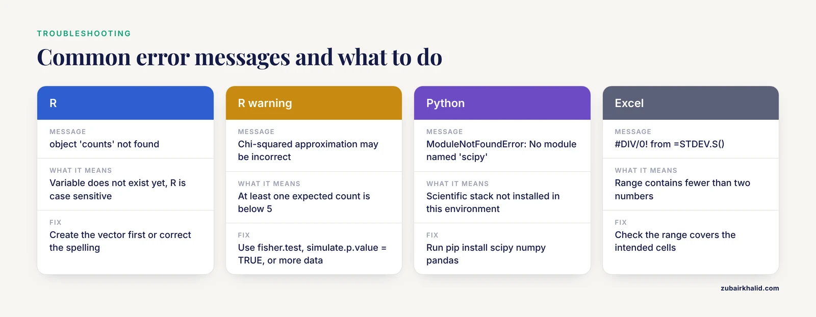
- Error: object 'counts' not found. The variable does not exist yet, and R is case sensitive. Create the vector first or correct the spelling.
- Chi-squared approximation may be incorrect (warning). At least one expected count is below 5. Use fisher.test for a 2x2 table, set simulate.p.value = TRUE, or collect more data.
- Error in t.test.default(...): data are essentially constant. One group has zero variance, usually because of repeated or mis-entered values. Inspect the raw numbers.
- ModuleNotFoundError: No module named 'scipy'. The Python scientific stack is not installed in the current environment. Run pip install scipy numpy pandas.
- #DIV/0! from =STDEV.S() in Excel. The range contains fewer than two numbers. Check that the range covers the intended cells.
Sensible next steps
Once single tests feel routine, move to linear models with lm(), learn a plotting system such as ggplot2, and put your scripts under version control. Those three moves turn a calculator into a workflow, and the workflow is what supervisors and reviewers actually want to see.
The Biology Calculator: Bench and Coursework Numbers
Some of the most frequent calculations in biology never involve a p-value. A biology calculator, whether a phone app, a web page, or a few lines of R, covers the routine arithmetic of the bench and the classroom.
Hardy-Weinberg proportions describe genotype frequencies in a population that is not evolving. If 4 percent of a population shows a recessive phenotype, then q² = 0.04, so q = 0.20 and p = 0.80, and the heterozygote frequency is 2pq = 0.32.
Solution preparation uses C1V1 = C2V2. To make 100 mL of 0.5 M NaCl from a 2 M stock, V1 = (0.5 × 100) / 2 = 25 mL of stock, diluted to a final volume of 100 mL.
Cell counts with a hemocytometer, dilution series, and standard curves follow the same pattern, and a spreadsheet handles all of them with transparent formulas. Build the habit from Step 4 above, compute each quantity once in the tool and once independently.
The Bioinformatics Calculator: Sequence and Alignment Numbers
A bioinformatics calculator computes quantities from sequence data. Most are descriptive, so know exactly what each one measures before you trust it.
GC content is the percentage of guanine and cytosine bases in a sequence. The 15-base read ATGGCCATTGGAATC contains 7 G or C bases out of 15, so GC = 7/15 = 46.7 percent.
Melting temperature (Tm) estimates the temperature at which half of a DNA duplex dissociates. For short oligonucleotides under about 14 bases, the Wallace rule gives Tm = 2 °C for each A or T plus 4 °C for each G or C. The 12-mer ATGCGGATCCGA has 4 A or T and 8 G or C, so Tm = (4 × 2) + (8 × 4) = 40 °C. Longer primers need salt-adjusted or nearest-neighbor formulas, which primer design tools implement for you.
Sequence search tools such as BLAST report an E-value, the expected number of matches scoring at least as well that chance alone would produce against a database of that size. An E-value of 0.001 means you would expect roughly one such match by chance per thousand searches of that size.
Beyond single sequences, scripted tools scale better. Biopython in Python and Bioconductor in R compute sequence statistics, read quality summaries, and differential expression tables from the same script that imports the raw data. Keep the descriptive layer separate from the statistical layer, because a GC content number is a summary, not a test.
Tips That Make Any Statistical Calculator More Trustworthy
- Script the analysis from day one. Even a single t-test belongs in a saved text file.
- Keep raw data read-only. All work happens on copies, and the raw file stays frozen.
- Fix your random seeds. If you simulate or bootstrap, set.seed(2026) in R makes the run repeatable.
- Record the environment. R's sessionInfo() prints the R and package versions, which belongs in your methods section or supplement.
- Cross-check at least one result per analysis by hand or with a second tool.
- Pre-specify the plan for formal studies. Registering a review protocol with PROSPERO before the searches begin, as the penile cancer quality-of-life review did, freezes the analysis plan and protects the findings from accusations of post hoc selection [2].
- Report effect sizes and intervals, not p-values alone.
Common Mistakes and Limitations
- Choosing the tool before the question. Software first leads you to whichever test the software makes easiest, which is rarely the test the design requires.
- Treating a click path as documentation. Point-and-click histories vanish, and six months later nobody can reconstruct which columns entered the model. Save the syntax or the script.
- Skipping assumption checks. The chi-square warning in Step 6 exists because the approximation degrades with small expected counts. Independence and approximate normality matter for t-tests and regression, and clustered data violate both.
- Reporting the unadjusted model because it looks better. In the frailty biomarker study described above, several blood and imaging markers appeared predictive in unadjusted models, and the associations disappeared after adjustment for age, sex, and other confounders [1]. The adjusted model answers the real question.
- Reading significance as importance. With enough subjects, a trivial difference produces a tiny p-value. The confidence interval tells the reader whether the effect is large enough to care about.
- Pooling without checking heterogeneity. In meta-analysis, large I² values mean the studies differ too much for one pooled number to describe them, and funnel plots with Egger's regression test probe whether small-study effects are inflating the pooled estimate [3].
- Expecting the calculator to rescue a weak design. No tool repairs confounding, missing data, or a sample too small for the question.
- One limitation deserves plain language: complex designs, clustered data, and nonlinear models justify a conversation with a consulting statistician before the data arrive, not after the first p-value.
Frequently Asked Questions
What is the best calculator for statistical analysis in research?
There is no single best tool. The best calculator for statistical analysis in research is the one that matches your design. For most life science work that means R or Python for the primary analysis, a spreadsheet for data entry, and a handheld or web calculator for quick checks.
Do I need paid software for publishable results?
No. R and Python are free, open-source, and used throughout the published life science literature. Paid packages add menus and support, not statistical validity.
Can Excel be my main statistical calculator?
For data entry, cleaning, and descriptive statistics, yes. For the primary inferential analysis of a study, use a dedicated package, because spreadsheet click paths make errors easy to commit and hard to detect.
What is a bioinformatics calculator?
It is a web tool or script that computes quantities from biological sequence data, such as GC content, melting temperature, molecular weight, and alignment E-values.
How do I calculate a p-value without software?
Compute the test statistic from its formula, then read the tail probability from a printed distribution table. That works for chi-square and small-sample t-tests, and it becomes impractical for regression or survival models.
Which calculator do I need for a meta-analysis?
Use RevMan or the metafor package in R. Whichever you choose must support the pooling method your protocol names, heterogeneity statistics such as I² and τ², and funnel plots.
How do I verify that my calculator gave the right answer?
Recompute one result with a second independent method, confirm the degrees of freedom and the sample counts, and check that the direction and size of the effect match the raw data.
What should a student learn first?
Learn spreadsheet basics, then R, starting with descriptive statistics, the chi-square test, the t-test, and linear models. Those four cover most undergraduate and early graduate analyses.
Sources
- Biological and Neuroimaging Markers as Predictors of 5-Year Incident Frailty in Older Adults: A Secondary Analysis of the MAPT Study.
- Quality-of-life Outcomes and Patient-reported Outcome Measures After Penile-preserving Surgery to Treat Penile Cancer: A Systematic Review and Meta-analysis.
- Pooled prevalence of infectious diseases among first responders in the prehospital setting: A systematic review with meta-analysis by occupation.