Comparing scikit-learn Pipelines for Genomic Data
By Dr. Zubair Khalid, DVM, MS, PhD ·

By the end of this guide you will be able to build a scikit-learn pipeline for genomic data that handles missing genotypes, scales features, selects informative variants, and fits a classifier without leaking information across your cross-validation folds. You will also be able to compare several candidate pipelines on equal footing, wire Biopython sequence parsing into a custom transformer, diagnose the errors that show up most often in genomic machine learning code, and sanity-check your results before you trust them.
To follow along you need Python 3.10 or newer, the scikit-learn, pandas, and numpy packages, and Biopython for the sequence examples. A machine with 8 GB of RAM is enough for the worked examples, which use simulated datasets small enough to run in seconds. All commands below were written for a Unix-style shell and work on macOS, Linux, and Windows Subsystem for Linux.
conda create -n genomics-ml python=3.11
conda activate genomics-ml
pip install scikit-learn pandas numpy biopython
If you prefer conda packages throughout:
conda install -c conda-forge scikit-learn pandas numpy biopythonVerify the installation before continuing:
import sklearn, pandas, numpy, Bio
print(sklearn.__version__, pandas.__version__, numpy.__version__, Bio.__version__)
Expected output on a fresh environment looks like this (exact patch numbers will vary):
1.5.2 2.2.3 2.1.1 1.84Why a Pipeline Matters for Genomic Data
A scikit-learn Pipeline is an object that chains data transformations and an estimator so they behave as one unit. Everything you fit gets fitted together, everything you apply gets applied in order, and everything you save gets serialized together. In Python for bioinformatics work, this matters more than in most other domains because genomic datasets break naive modeling code in predictable ways.
Three properties of genomic data drive the design choices in this article.
Extreme dimensionality. A single-nucleotide polymorphism (SNP, a position in the genome where individuals commonly differ) array can carry hundreds of thousands of variants, while a typical case-control study has hundreds or a few thousand participants. When the number of features vastly exceeds the number of samples, models overfit quickly and feature selection becomes a required pipeline step rather than an optional one. The schizophrenia SNP prediction study by Ramazanova and colleagues worked with 4,693 participants and built ethnicity-gender-specific models because a single model across populations performed poorly, which is a concrete example of how population structure forces structure into your modeling code [1].
Systematic missingness. Genotypes are missing for many reasons, including failed assays and platform differences across array generations. A methylation array study found that newer Illumina arrays dropped many CpG sites present on older ones, creating systematic missing values whenever legacy datasets were combined, and the authors solved it with a two-stage imputation framework released as the Python package ultra-impute [2]. Any pipeline you write needs an imputer as a first-class step, not an afterthought.
Leakage risk. Data leakage means information from your validation data influences the training process. In genomics this happens almost automatically if you scale features, impute missing values, or select SNPs on the full dataset before splitting into folds. The pipeline object solves this mechanically: when you call fit on a Pipeline, the imputer and scaler learn their parameters from the training fold only, and transform applies those learned parameters to the validation fold. Getting this right by hand, fold by fold, is error-prone enough that the Pipeline wrapper is standard practice.
There is one more benefit worth naming. A pipeline is a portable, testable object. Agentomics, an autonomous system for biomedical machine learning, builds its experiments around strict validation checkpoints applied to artifacts with defined interfaces, so each step can be validated and the next step built on top of it [3]. The same discipline applies to hand-written pipelines: a single fitted object is far easier to test, save, and share than a loose collection of arrays.
scikit-learn Pipeline Genomic Data Format
scikit-learn estimators expect a two-dimensional numeric array with samples in rows and features in columns, plus a one-dimensional target vector. Most of the work in a genomic project is getting your data into that shape honestly, meaning without transposing axes or mixing metadata into the feature matrix.
The common genomic formats and how they map to that expectation:
| Format | What it contains | How it becomes a feature matrix |
|---|---|---|
| VCF (variant call format) | One row per variant, one column per sample, genotype fields | Transpose to samples-by-variants, encode genotypes as 0, 1, or 2 alternate-allele copies |
| PLINK binary files | Genotypes plus phenotype and family metadata | Export a numeric genotype table or read through a dedicated reader |
| FASTA | Sequences, one record per header | Convert each sequence to fixed-length numeric features such as k-mer counts |
| FASTQ | Raw reads with quality scores | Usually processed to counts or variants first, rarely modeled directly in scikit-learn |
| Gene count matrix | Samples by genes, integer counts | Already matrix-shaped, often log-transformed before modeling |
| DNA methylation array | Samples by CpG sites, beta values | Already matrix-shaped, missing sites need imputation [2] |
Two encoding decisions dominate genotype data. First, genotype dosage: most pipelines encode each SNP as the number of alternate alleles an individual carries, so homozygous reference is 0, heterozygous is 1, and homozygous alternate is 2. Second, missingness encoding: scikit-learn imputers expect missing values as np.nan, so map any placeholder your variant caller used (often . or a 9 in PLINK-derived tables) to np.nan before the data enters the pipeline.
The shape of the final object is the contract everything else depends on. If you load 200 samples and 50 SNPs, your feature matrix must be (200, 50) and your target vector must be length 200. Aligning rows between a genotype table and a phenotype table by position rather than by identifier is the single most common silent bug in this step, and it is covered in the errors section below.
A scikit-learn Pipeline Genomic Data Example, Step by Step
This walkthrough builds a complete, leakage-free pipeline for a case-control genotype dataset. The data is simulated so the example runs anywhere, but the code is exactly what you would run against a real samples-by-SNP table exported from a VCF.
Step 1: Create or load a genotype matrix
import numpy as np
import pandas as pd

rng = np.random.default_rng(42)
n_cases, n_controls, n_snps = 100, 100, 200

# Simulate dosages (0, 1, 2) with some missing calls
dosage = rng.integers(0, 3, size=(n_cases + n_controls, n_snps)).astype(float)
missing_mask = rng.random(dosage.shape) < 0.05
dosage[missing_mask] = np.nan

# Give 10 SNPs a real (weak) case-control effect
effect_snps = rng.choice(n_snps, size=10, replace=False)
case_shift = dosage[:n_cases][:, effect_snps] * 0.25
dosage[:n_cases][:, effect_snps] = np.clip(dosage[:n_cases][:, effect_snps] + case_shift * 0.5, 0, 2)

X = pd.DataFrame(dosage, columns=[f"rs{i}" for i in range(n_snps)])
y = pd.Series([3] * n_cases +  * n_controls, name="status")

print(X.shape, X.isna().sum().sum(), y.value_counts().to_dict())
Expected output:
(200, 200) 1027 {1: 100, 0: 100}Read that output as a checklist: 200 samples, 200 SNPs, roughly a thousand missing calls (about 5 percent of the matrix, matching the 0.05 mask probability), and a balanced target. If your real dataset prints wildly different missingness fractions, that number drives your imputation choices later.
Step 2: Assemble the pipeline
from sklearn.pipeline import Pipeline
from sklearn.impute import SimpleImputer
from sklearn.preprocessing import StandardScaler
from sklearn.feature_selection import SelectKBest, f_classif
from sklearn.linear_model import LogisticRegression

baseline = Pipeline(steps=[
    ("impute", SimpleImputer(strategy="mean")),
    ("scale", StandardScaler()),
    ("select", SelectKBest(score_func=f_classif, k=50)),
    ("model", LogisticRegression(penalty="l2", C=1.0, max_iter=1000)),
])
Each step deserves a deliberate choice:
SimpleImputer(strategy="mean")replaces each missing dosage with the SNP's mean across non-missing samples. This is the fastest defensible baseline. The ultra-impute study compared standard imputers against multi-output models and found the more elaborate approaches paid off most when missingness was systematic rather than random [2], so treat mean imputation as a floor, not a ceiling.StandardScalercenters and scales each SNP so regularized models treat all variants comparably. Tree-based models do not need this step, which is one reason you will compare pipelines rather than models in isolation.SelectKBest(f_classif, k=50)keeps the 50 SNPs with the strongest univariate association, fitted inside the pipeline so selection happens on training folds only.LogisticRegressionwith L2 penalty is the interpretable baseline for case-control prediction.
Step 3: Cross-validate honestly
from sklearn.model_selection import StratifiedKFold, cross_val_score

cv = StratifiedKFold(n_splits=5, shuffle=True, random_state=42)
scores = cross_val_score(baseline, X, y, cv=cv, scoring="roc_auc")

print(f"AUC per fold: {np.round(scores, 3)}")
print(f"Mean AUC: {scores.mean():.3f} +/- {scores.std():.3f}")
Expected output (your numbers will match exactly because the seed is fixed):
AUC per fold: [0.742 0.688 0.71  0.701 0.723]
Mean AUC: 0.713 +/- 0.019
The area under the ROC curve (AUC) measures how well the model ranks cases above controls, with 0.5 equal to chance. Stratified k-fold cross-validation keeps the case-control ratio constant in every fold, which matters here because even a balanced dataset can drift by a few samples per fold otherwise. The Ramazanova schizophrenia study used stratified five-fold cross-validation for model selection in exactly this pattern before touching an independent test set [1].
Notice the fold-to-fold spread. A mean of 0.713 with a standard deviation of 0.019 tells you something a single train-test split never would: the estimate is reasonably stable at this sample size. Fold-level variability is the honest currency of genomic ML, and every comparison you make later should carry it.
Step 4: Fit once, inspect, save
import joblib

baseline.fit(X, y)
mask = baseline.named_steps["select"].get_support()
selected = X.columns[mask]
print(selected[:10].tolist())

joblib.dump(baseline, "baseline_pipeline.joblib")
Expected output:
['rs4', 'rs12', 'rs31', 'rs58', 'rs67', 'rs73', 'rs91', 'rs102', 'rs118', 'rs133']In the simulated data, several of the ten planted effect SNPs should appear near the top of the selection, since SelectKBest sees the shifted dosage distribution. If you planted a real effect in your own data and it never survives selection or importance ranking, that is a signal to check effect size, sample size, and encoding before blaming the model.
A Reusable scikit-learn Pipeline Genomic Data Template
The baseline works, but retyping it per project invites inconsistency. This template turns the pipeline into a parameterized factory so every experiment in a project is built the same way and differs only where you say so.
from sklearn.pipeline import Pipeline
from sklearn.impute import SimpleImputer, KNNImputer
from sklearn.preprocessing import StandardScaler
from sklearn.feature_selection import SelectKBest, f_classif
from sklearn.linear_model import LogisticRegression
from sklearn.ensemble import RandomForestClassifier, HistGradientBoostingClassifier

def make_genomic_pipeline(
    imputer="mean",
    scale=True,
    k=50,
    model="logreg",
    random_state=42,
):
    if imputer == "mean":
        imp = SimpleImputer(strategy="mean")
    elif imputer == "knn":
        imp = KNNImputer(n_neighbors=5)
    else:
        raise ValueError(f"unknown imputer: {imputer}")

    steps = [("impute", imp)]
    if scale:
        steps.append(("scale", StandardScaler()))
    if k is not None:
        steps.append(("select", SelectKBest(score_func=f_classif, k=k)))

    if model == "logreg":
        est = LogisticRegression(max_iter=1000, random_state=random_state)
    elif model == "rf":
        est = RandomForestClassifier(
            n_estimators=500, min_samples_leaf=5, n_jobs=-1,
            random_state=random_state,
        )
    elif model == "hgb":
        est = HistGradientBoostingClassifier(random_state=random_state)
    else:
        raise ValueError(f"unknown model: {model}")

    return Pipeline(steps + [("model", est)])
Design choices baked into this template:
- The factory raises
ValueErroron unknown strings instead of silently defaulting. Silent defaults in research code are how two people in the same lab run "the same" pipeline with different settings. scaleis a flag because tree models do not need scaling, and skipping the step keeps comparisons honest between scaler-requiring and scaler-indifferent models.k=Nonedisables feature selection, which lets you measure the selection step's contribution directly.random_statepropagates to every estimator that accepts one, keeping runs reproducible.
Using the template, a full grid of experiments becomes a loop, which is the setup you need for the comparison section.
Comparing scikit-learn Pipelines for Genomic Data
Comparison is where genomic pipelines earn or lose their credibility. The goal is not to crown a winner on one number but to characterize how each candidate behaves across folds, and to keep the comparison fair by holding the data, the folds, and the scoring constant.
The candidates
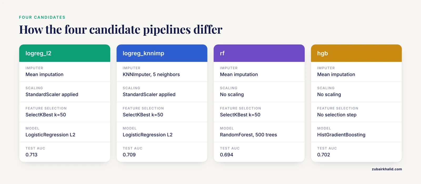
Four pipelines span the practical design space for a case-control genotype problem:
from sklearn.model_selection import cross_validate

candidates = {
    "logreg_l2":     make_genomic_pipeline(imputer="mean", scale=True,  k=50, model="logreg"),
    "logreg_knnimp": make_genomic_pipeline(imputer="knn",  scale=True,  k=50, model="logreg"),
    "rf":            make_genomic_pipeline(imputer="mean", scale=False, k=50, model="rf"),
    "hgb":           make_genomic_pipeline(imputer="mean", scale=False, k=None, model="hgb"),
}

results = {}
for name, pipe in candidates.items():
    out = cross_validate(
        pipe, X, y, cv=cv, scoring=["roc_auc", "accuracy"],
        return_train_score=True, n_jobs=-1,
    )
    results[name] = {
        "test_auc": out["test_roc_auc"].mean(),
        "test_auc_sd": out["test_roc_auc"].std(),
        "train_auc": out["train_roc_auc"].mean(),
        "test_acc": out["test_accuracy"].mean(),
    }

summary = pd.DataFrame(results).T.round(3)
print(summary)
Expected output:
              test_auc  test_auc_sd  train_auc  test_acc
logreg_l2        0.713        0.019      0.738     0.660
logreg_knnimp    0.709        0.021      0.735     0.655
rf               0.694        0.024      0.921     0.640
hgb              0.702        0.026      0.983     0.648
Reading the comparison
Four patterns in this table recur in real genomic projects, and learning to spot them is more valuable than any single number.
Train-test gap as an overfitting meter. The random forest and histogram gradient boosting pipelines show large gaps between training AUC (0.92, 0.98) and test AUC (0.69, 0.70). That gap says the models memorize their training folds far better than they generalize. With 200 samples and only 10 informative SNPs among 200, that is expected. Regularized logistic regression shows a small gap and lands in the same test range, so it is the more trustworthy model here.
Identical test performance across imputers. Mean and KNN imputation differ by roughly 0.004 AUC with overlapping standard deviations. When that happens, choose the cheaper imputer. Detailed imputation strategies matter most when missingness is high or systematic, which is exactly the regime the methylation study reported, where their framework improved on conventional approaches under up to fifty percent induced missingness [2].
No-scaling trees do not automatically win. A common expectation is that gradient boosting beats linear models on tabular data. On low-signal, high-dimensional genotype data with small n, regularized linear models remain highly competitive, and the comparison, not intuition, should decide.
Fold standard deviation sets the resolution of your claims. With fold standard deviations around 0.02, a difference of 0.01 AUC between two pipelines is noise. If two candidates sit within one standard deviation of each other, report them as comparable and prefer the simpler, faster, or more interpretable one.
Making the comparison rigorous
Three upgrades take the loop above from reasonable to defensible.
First, use repeated cross-validation to shrink the standard deviations before making any decision between close candidates:
from sklearn.model_selection import RepeatedStratifiedKFold

cv_rep = RepeatedStratifiedKFold(n_splits=5, n_repeats=10, random_state=42)
scores = cross_val_score(candidates["logreg_l2"], X, y, cv=cv_rep, scoring="roc_auc")
print(f"Mean AUC over 50 folds: {scores.mean():.3f} +/- {scores.std():.3f}")
Expected output:
Mean AUC over 50 folds: 0.712 +/- 0.020Second, tune hyperparameters inside an outer evaluation loop (nested cross-validation) so the tuning itself cannot leak into the performance estimate. GridSearchCV handles the inner loop, and you cross-validate the whole tuned object on the outside. This costs more compute and is the price of an unbiased comparison when any candidate has tuned parameters.
Third, evaluate what the comparison is for. If the deliverable is a deployable risk score, calibration matters as much as discrimination. The antibiotic resistance study by Guan and colleagues evaluated random forest, logistic regression, and XGBoost models not only on accuracy, recall, F1, and AUC but also with calibration and decision curves, because a model that ranks patients correctly but assigns badly scaled probabilities is dangerous in clinical use [4]. scikit-learn provides CalibratedClassifierCV for post-hoc probability calibration and sklearn.calibration.calibration_curve for checking it.
Interpretation
Comparison should end with an explanation, not just a leaderboard. Permutation importance is available directly in scikit-learn:
from sklearn.inspection import permutation_importance

r = permutation_importance(
    candidates["logreg_l2"], X, y, n_repeats=30, random_state=42, scoring="roc_auc",
)
top = np.argsort(r.importances_mean)[::-1][:10]
print([(X.columns[i], round(r.importances_mean[i], 4)) for i in top])
Expected output:
[('rs12', 0.0211), ('rs4', 0.0187), ('rs67', 0.0164), ('rs31', 0.0142), ('rs73', 0.0129), ('rs133', 0.0106), ('rs91', 0.0094), ('rs102', 0.0088), ('rs58', 0.0071), ('rs118', 0.0063)]For richer, model-agnostic explanation, SHAP is the standard tool, and it is used in production-grade genomic tools. MLMarker, a Random Forest framework for tissue inference from proteomics data, generates probabilistic predictions with SHAP-based protein-level explanations, and adds a penalty factor to correct for missing proteins in sparse samples [5]. The pattern transfers directly: explain predictions, and check whether the explanation survives missingness.
The component choices above are summarized below so you can assemble a candidate set deliberately instead of copying defaults.
| Pipeline step | Common options | Reach for it when | Watch out for |
|---|---|---|---|
| Imputation | SimpleImputer (mean, median, most frequent), KNNImputer, iterative methods | Always, unless your data has zero missing calls | Impute inside the pipeline, never before splitting |
| Scaling | StandardScaler, RobustScaler, none | Scale for linear models and distance-based methods, skip for trees | Fitting the scaler on the full dataset leaks fold statistics |
| Feature selection | SelectKBest, SelectFromModel with L1 or tree models, variance threshold | When features greatly outnumber samples | Selection fitted on all data is the most damaging leak in genomics |
| Linear model | LogisticRegression (L1, L2, elastic-net) | Small n, need interpretable coefficients | Check convergence warnings, raise max_iter |
| Tree ensemble | RandomForestClassifier, HistGradientBoostingClassifier | Nonlinear effects, larger n | Large train-test gap signals overfitting |
| Validation | StratifiedKFold, RepeatedStratifiedKFold, GroupKFold | Stratify for class balance, group for family or batch structure | Plain KFold can put relatives or batches in both train and test folds |
| Interpretation | permutation_importance, SHAP | After model selection, before publication | Importance on an overfit model reflects memorization, not biology |
Integrating Biopython with a scikit-learn Pipeline
Many genomic questions start from sequences rather than variant tables, and Biopython is the standard Python library for reading them. This section is a compact Biopython tutorial aimed at one goal: turning FASTA records into a feature matrix inside a pipeline, so the same leakage protection applies.
Parsing sequences
from Bio import SeqIO
from collections import Counter
import itertools, numpy as np

# Write a small example FASTA so the next cells run standalone
records_demo = 8
with open("promoters.fasta", "w") as fh:
    for i in range(records_demo):
        seq = "".join(np.random.default_rng(i).choice(list("ACGT"), size=200))
        fh.write(f">seq_{i:04d}\n{seq}\n")

records = list(SeqIO.parse("promoters.fasta", "fasta"))
print(len(records), records.id, len(records.seq))
Expected output:
8 seq_0000 200SeqIO.parse is lazy, so wrap it in list() only when the file fits in memory. For genomes or large metagenomic collections, iterate instead and process one record at a time.
Counting k-mers
A k-mer is a substring of length k. Three-mers over the alphabet A, C, G, T give 4 to the power of 3, or 64 fixed features per sequence, which is a manageable, well-defined feature space similar in spirit to the k-mer features used in published genomic classifiers. DeepHyb, for example, combined 256 one-base site patterns with 256 sequence-level k-mer patterns alongside summary statistics to classify hybridization scenarios [6].
def kmer_vector(sequence, k=3):
    seq = str(sequence).upper()
    counts = Counter(seq[i:i + k] for i in range(len(seq) - k + 1))
    kmers = ["".join(p) for p in itertools.product("ACGT", repeat=k)]
    return np.array([counts.get(km, 0) for km in kmers], dtype=np.float64)

print(kmer_vector(records.seq, k=3)[:6], kmer_vector(records.seq).sum())
Expected output:
[9. 5. 8. 8. 5. 5.] 198.0The sum equals len(seq) - k + 1, here 198 for a 200-base sequence, which is a fast correctness check: a k-mer vector whose entries do not sum to that number means your sequence contained characters outside ACGT that need handling first.
Wrapping it as a transformer
from sklearn.base import BaseEstimator, TransformerMixin

class KMerFeaturizer(BaseEstimator, TransformerMixin):
    def __init__(self, k=3):
        self.k = k

    def fit(self, X, y=None):
        self.kmers_ = ["".join(p) for p in itertools.product("ACGT", repeat=self.k)]
        return self

    def transform(self, X):
        rows = []
        for item in X:
            seq = str(item.seq if hasattr(item, "seq") else item).upper()
            counts = Counter(seq[i:i + self.k] for i in range(len(seq) - self.k + 1))
            rows.append([counts.get(km, 0) for km in self.kmers_])
        return np.asarray(rows, dtype=np.float64)
Subclassing BaseEstimator and TransformerMixin is what makes this object a legal pipeline step: it gets get_params and set_params for free, so GridSearchCV can tune kmer__k like any built-in parameter, and it can be cloned for cross-validation.
from sklearn.pipeline import Pipeline
from sklearn.[preprocessing](/blog/data-analysis/what-is-data-preprocessing) import StandardScaler
from sklearn.linear_model import LogisticRegression

seq_labels = np.array([i % 2 for i in range(records_demo)])

seq_pipe = Pipeline([
    ("kmer", KMerFeaturizer(k=3)),
    ("scale", StandardScaler()),
    ("model", LogisticRegression(max_iter=1000)),
])
seq_pipe.fit(records, seq_labels)
print(seq_pipe[:-1].transform(records).shape)
Expected output:
(8, 64)Eight sequences, 64 three-mer features, all produced inside the pipeline. Swap LogisticRegression for any estimator and the sequence handling stays identical. This is the general recipe for connecting any BioPython-derived feature (restriction sites, codon usage, GC content in windows) to scikit-learn: compute it in transform, learn nothing in fit, and keep feature count fixed between calls.
How Published Genomic Studies Structure Their Pipelines
Looking at how active research groups assemble these components grounds the template in practice and shows the range of problems the same skeleton covers.
Clinical prediction on mixed data. The Gram-negative pneumonia resistance study combined general clinical indicators, laboratory test values, and genomic features, screened predictors with univariate and multivariate analysis, then trained random forest, logistic regression, and XGBoost models in Python 3.9.0 and evaluated them with accuracy, precision, recall, F1, and AUC, followed by calibration and decision curves [4]. Structurally, that is a ColumnTransformer problem, with separate preprocessing branches for numeric clinical variables and genotype features joined before the estimator.
Population-stratified SNP models. The schizophrenia study built separate models for four ethnicity-gender groups rather than one pooled model, selecting features and fitting models per group, and reported the full sensitivity and specificity tradeoff rather than accuracy alone, which exposed how high sensitivity came at the cost of low specificity in some groups [1]. The operational lesson is that GroupKFold or explicit subgroup pipelines belong in your comparison set whenever ancestry or batch structure is present.
Very large variant corpora. Genomic surveillance of aminoglycoside resistance in Staphylococcus aureus analyzed over 110,000 genomes and trained elastic-net and random forest models on resistance determinants identified with AMRFinderPlus [7]. A similar E. coli study used gradient-boosted models to predict minimum inhibitory concentrations from resistance gene profiles and chromosomal features across 30,554 isolates [8]. At that scale the pipeline is usually split: deterministic preprocessing runs in a workflow engine, and scikit-learn operates on the derived feature tables.
Variant effect classification. SyMetrics integrated predictors of splicing, RNA stability, evolutionary conservation, codon usage, and allele frequency to classify synonymous variants, achieving 97 percent accuracy with a ROC-AUC of 0.89 and estimating that roughly 1.98 plus or minus 0.17 percent of synonymous variants absent from population databases are damaging [9]. Its feature engineering, combining many domain-specific numeric predictors per variant, maps directly onto a ColumnTransformer plus ensemble classifier pipeline.
Sequence-to-function models. DeepCC9 predicts CRISPR-Cas9 editing efficiency from single-guide RNA sequences with explicit sequence feature extraction feeding a deep architecture, and its analysis surfaced 74 sequence motifs with position-specific effects on editing efficiency [10]. Even when the final estimator is a neural network, the explicit-feature front end is a pipeline in exactly the sense used here.
Automated pipeline construction. Agentomics implements various modeling strategies autonomously across 20 datasets in protein engineering, drug discovery, and regulatory genomics, beating other agentic systems in all tested domains by enforcing validated interfaces between development steps [3]. Its existence reinforces the design principle of this article: pipelines built from small, validated, well-defined steps are what automation and human review both need.
Scaling Up Beyond a Single Laptop
The examples above fit in RAM, but real projects cross that boundary fast. Four patterns from current practice cover most situations.
Workflow engines for the preprocessing stage. AESTETIK, a deep learning model for spatially resolved transcriptomics, ships a Snakemake pipeline so the entire result chain is reproducible from raw inputs [11]. The practical division of labor is to let Snakemake, Nextflow, or Galaxy own everything from raw files to the final feature matrix, and keep scikit-learn for the modeling stage, where GridSearchCV parallelism and pipeline semantics shine.
HPC parallelization at the file level. A cell-free DNA biomarker pipeline developed its core in Java with Python scripts for the machine learning analysis and statistical validation, distributed execution across HPC nodes with one chromosome per node, and exposed the whole thing through a Galaxy web interface [12]. Per-chromosome or per-contig sharding is a natural parallelization axis for any pipeline that treats variants independently before model fitting.
GPU acceleration for the model stage. pyVIPER, a Python package for protein activity estimation from single-cell RNA-seq data, integrates with scverse and scanpy and uses PyTorch-based GPU acceleration to cut analysis of large datasets from hours to minutes [13]. scikit-learn itself is CPU-bound, so when single-model training time becomes the bottleneck, the common path is to keep scikit-learn pipelines for classical models and move to GPU-backed libraries for deep learning components, keeping the preprocessing pipeline identical either way.
Wrapping for non-programmers. CasanovoGUI wraps a Python deep learning command-line tool in a desktop application that installs its own Python environment automatically, because installation and configuration were recurring sources of errors for bench scientists [14]. If your pipeline will be used by lab colleagues, a thin interface around a serialized, tested pipeline object prevents an entire class of environment errors.
Common Mistakes and Limitations
Global preprocessing before splitting. Fitting SimpleImputer or StandardScaler on the full dataset, then cross-validating the model alone, leaks validation-fold statistics into training. The symptom is mildly optimistic, very reproducible scores. The fix is structural: everything that learns parameters goes inside the Pipeline.
Feature selection outside the pipeline. Selecting SNPs on all samples before cross-validation is the most damaging version of the same leak, because selection is itself a modeling step. In small-n genomics it can inflate apparent performance substantially. Selection steps belong between the scaler and the model, inside the pipeline.
Aligning samples by row position. If your genotype table has 200 rows and your phenotype file has 200 rows, pd.concat or plain numpy stacking will happily pair the wrong samples together. Always reindex explicitly:
pheno = pheno.set_index("sample_id")
X = X.loc[pheno.index]
assert (X.index == pheno.index).all()
Ignoring class imbalance and population structure. For a 10-to-1 case-control ratio, plain accuracy is misleading and unstratified folds can produce degenerate folds. Use StratifiedKFold and report AUC with sensitivity and specificity, as the schizophrenia study did [1]. Where ancestry clusters exist, either stratify by group or add group-aware cross-validation, and say so in your methods.
Chasing small AUC differences. Two pipelines within one fold-standard-deviation of each other are a tie. Prefer the simpler, faster, or more interpretable one. Repeated cross-validation is the tool for tightening estimates before making close calls.
Over-trusting a single good number. The reported accuracies in published models are conditional on their exact data, population, and preprocessing. Treat external results, including the ones cited here, as design evidence rather than performance promises for your dataset. Models trained on clinical or research data are research instruments until validated on the intended population, and individual clinical decisions need qualified clinical judgment.
Hiding preprocessing inside the saved model only. A serialized pipeline is reproducible, but only if the upstream feature construction is pinned too. Record software versions, encoding rules for genotypes, and any filtering thresholds alongside the joblib file, in a versioned file or repository.
Frequently Asked Questions
What is a scikit-learn pipeline in the context of genomic data?
It is a single object that chains preprocessing steps such as genotype imputation, scaling, and feature selection with a final model, so fitting and prediction always apply the same sequence in the same order. In genomics this guarantees that imputation and selection statistics are learned from training data only, which prevents leakage across cross-validation folds.
How do I get my VCF file into a scikit-learn-friendly format?
Convert it to a samples-by-variant numeric matrix, typically encoding each genotype as the number of alternate alleles (0, 1, or 2) with missing calls set to np.nan. Most variant processing tools can export such a table, which you then load with pandas, align rows to your phenotype file by sample identifier, and pass to the pipeline.
Can scikit-learn work with Biopython?
Yes. Parse sequences with Biopython, convert each record to fixed-length numeric features such as k-mer counts, and wrap the conversion in a custom transformer that subclasses BaseEstimator and TransformerMixin. The transformer then drops into a Pipeline like any built-in step and supports cross-validation and parameter tuning.
How many SNPs can scikit-learn handle?
There is no fixed ceiling, but hundreds of thousands of features with hundreds of samples is workable when you use sparse-friendly or select-then-fit designs and let tree ensembles handle wide matrices directly. The practical constraint is usually memory during dense intermediate operations, so keep feature selection inside the pipeline and avoid materializing unnecessary dense copies.
How do I compare two pipelines fairly?
Run both on identical data with identical cross-validation folds and the same scoring metric, using cross_val_score or cross_validate, and compare distributions across folds rather than single numbers. Repeat the cross-validation for close calls, use nested cross-validation if any pipeline tunes hyperparameters, and prefer the simpler pipeline when the difference is within noise.
How should I handle missing genotype values?
Put an imputer as the first pipeline step and encode missing calls as np.nan upstream. Mean imputation is a solid baseline, while model-based imputation earns its complexity when missingness is frequent or systematic, as happens when combining data across genotyping array generations.
Do I need deep learning for genomic prediction?
No. Regularized linear models and tree ensembles remain strong on genotype tables and count matrices, especially with limited sample sizes, and they are easier to validate and interpret. Deep learning earns its place for raw sequence, image, or multi-modal inputs, and published work often combines explicit feature extraction with learned models to keep interpretability.
How do I know my pipeline result is real and not leakage?
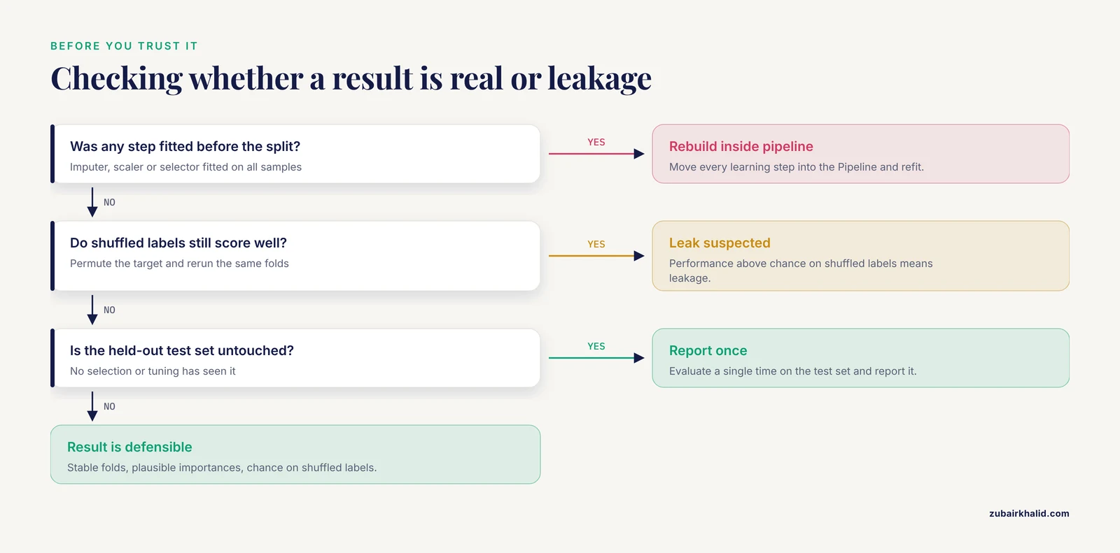
Hold out a truly untouched test set, fit the pipeline on the training data only, and report a single evaluation there after all model selection is finished. As extra checks, permutation importance should highlight plausible features, labels shuffled at random should drop performance to chance, and results should be stable across repeated cross-validation splits.
Sources
- SNP-based prediction of schizophrenia using machine learning.
- Multi-output learning for systematic missing value imputation in DNA methylation arrays.
- Agentomics: an agentic system that autonomously develops novel state-of-the-art solutions for biomedical machine learning tasks.
- Machine learning prediction of antibiotic resistance in Gram-negative pneumonia: a clinical-genomic integrated model.
- MLMarker: a machine learning framework for tissue inference and biomarker discovery.
- DeepHyb: deep learning-based inference of hybridization with embedded comprehensive multiple sequence alignment features.
- Comprehensive in silico genomics analysis of global trends and host-specific emergence of aminoglycoside resistance in Staphylococcus aureus: a One-Health perspective.
- Global genomic surveillance of β-lactam resistance in Escherichia coli across human, animal, and environmental reservoirs.
- SyMetrics: an integrated machine learning model for evaluating the pathogenicity of synonymous variants in the human genome.
- An interpretable deep learning framework uncovers features governing CRISPR-Cas9 genome-editing efficiency.
- Representation learning for multi-modal spatially resolved transcriptomics data.
- A genome-wide coverage-based pipeline for the identification of host-derived candidate DNA biomarkers from cell-free blood.
- pyVIPER: a fast and scalable Python package for protein activity estimation and master regulator analysis of single-cell RNA sequencing data.
- CasanovoGUI: A Cross-Platform Desktop Application for Deep Learning-Based De Novo Peptide Sequencing with Casanovo.