RNA-seq TPM vs RPKM: How to Choose
By Dr. Zubair Khalid, DVM, MS, PhD ·

TPM (transcripts per million) rescales each gene's length-corrected read count against the sum of all length-corrected counts in the same sample, so every sample totals exactly one million, while RPKM (reads per kilobase per million) rescales against the raw library size and lets each sample's total drift. That single difference in the order of operations is the whole story. The rule of thumb: use TPM when you need gene-level expression values that are comparable across samples, use RPKM or FPKM only for compatibility with legacy datasets, and use neither for differential expression testing, where raw counts with count-based normalization win. If you remember nothing else from this article, remember that the difference between RNA-seq TPM and RPKM is not the gene length correction. Both correct for gene length. The difference is what happens after it.
What TPM and RPKM Actually Measure
RNA-seq gives you raw counts: the number of reads or fragments assigned to each gene in each sample. Raw counts are confounded by two technical factors before they say anything about biology. First, samples are sequenced to different depths, so a gene in a deeply sequenced sample accumulates more reads even at identical expression. Second, longer genes capture more reads at the same molar concentration, so count magnitude partly reflects transcript length rather than abundance. RPKM, FPKM, and TPM are three attempts to remove both effects, and they differ only in the sequence of steps.
RPKM and FPKM
RPKM for a gene is computed as:
RPKM = (gene reads × 10^9) / (total mapped reads × gene length in bp)
Equivalently, divide the gene's read count by its length in kilobases, then divide by the library size expressed in millions of mapped reads. The "per million" denominator is the total number of mapped reads in that sample. FPKM is the paired-end version: fragments, which correspond to cDNA molecules, replace reads, and a fragment spanning two exons is counted once even though both mates map there. For single-end data, FPKM and RPKM are numerically identical.
The critical property of RPKM is what the "per million" refers to. It refers to the raw library size, the number of reads you actually sequenced. That number is a property of the sequencing run, not of the transcriptome, and this is where the trouble begins.
TPM
TPM reorders the steps:
- Divide each gene's read count by its length in kilobases to get reads per kilobase (RPK).
- Sum the RPK values across all genes in that sample.
- Divide each gene's RPK by that sum and multiply by 10^6.
TPM = (gene RPK / sum of all RPK in the sample) × 10^6
The "per million" in TPM refers to a length-corrected transcript pool within the sample, not to the sequenced reads. Because of this, the TPM values in every sample sum to exactly one million, which makes each TPM interpretable as a share of the sample's total transcript pool, adjusted for gene length.
The Order of Operations Is the Whole Difference
The difference between RNA-seq TPM and RPKM comes down to which denominator is applied last. In RPKM, the final scaling factor is the library size, so a sample whose reads are concentrated in a few long, highly expressed genes will have a smaller sum of RPKM values across genes, and the remaining genes will carry deflated RPKM values relative to an otherwise identical sample. In TPM, the final scaling factor is the sum of length-corrected counts, so the totals are pinned to one million by construction and each value is a relative molar share.
This ordering problem is not unique to RPKM. It is a general compositional problem in sequencing data. Robinson and Oshlack demonstrated that when a subset of genes consumes a large fraction of the reads in one condition, plain library-size normalization absorbs the compositional shift and produces biased fold changes, and they proposed the trimmed mean of M values (TMM) method to correct for it [1]. TPM reduces, but does not eliminate, exposure to the same compositional effect, because forcing the totals to one million still makes all values relative. Any normalization built on RNA-seq count data lives inside a compositional constraint, and you should interpret both TPM and RPKM with that in mind.
Side-by-Side Comparison
| Feature | TPM | RPKM | FPKM |
|---|---|---|---|
| What it measures | Relative molar share of a transcript in the sample's RNA pool, length-corrected | Reads per kilobase of transcript per million mapped reads | Fragments per kilobase per million mapped reads (paired-end) |
| Length correction | Applied first | Applied first | Applied first |
| Final scaling denominator | Sum of length-corrected counts in the same sample | Raw library size (mapped reads) | Raw library size (mapped fragments) |
| Sum across genes per sample | Always 10^6 in every sample | Varies from sample to sample | Varies from sample to sample |
| Comparable across samples at the gene level | Yes, with the compositional caveat | No, totals drift with sample composition | No, same problem as RPKM |
| Meaning of an identical value in two samples | Same share of the transcript pool | Not the same share, denominators differ | Not the same share |
| Paired-end handling | Works with fragments if you feed fragment counts | Not appropriate, counts mates twice conceptually | Designed for paired-end data |
| Suitable input for DE testing | No, use raw counts with count-based normalization | No | No |
| Current status | Recommended for cross-sample gene-level reporting | Legacy, single-end era | Legacy, Cufflinks-era standard |
The row that settles most arguments is the "sum across genes" row. If TPMs sum to one million in every sample, then a TPM of 500 means the same thing in sample A and sample B. If RPKM sums differ between samples, an RPKM of 500 in one sample and 500 in another do not describe the same fraction of anything.
TPM in Practice
TPM answers one question cleanly: of all the transcripts in this sample, what fraction does this gene represent, accounting for the fact that longer genes capture more reads? Because the answer is expressed on a fixed scale, TPM is the right unit for a specific and common set of tasks.
When to use RNA-seq TPM:
- Comparing the expression of the same gene across many samples, for example a heatmap of one signature across a cohort, a boxplot of a single gene across tissue types, or a dot plot of marker genes per cell type.
- Comparing expression levels between genes within a sample, for example ranking the ten most abundant transcripts in a tissue. Without length correction this comparison is meaningless, and TPM provides it on a stable scale.
- Feeding a fixed-scale expression matrix into methods that assume comparability across samples, such as visualization, clustering of samples, and some machine learning pipelines.
- Thresholding for presence or absence calls in reporting, for example filtering genes below a TPM cutoff across samples before stating that a transcript is detectably expressed. Thresholds should be justified per dataset, not copied blindly.
- Building tissue or condition-specific resources where downstream tools expect relative abundance as input. Benchmarking of genome-scale metabolic model construction compared TPM, FPKM, TMM, GeTMM, and RLE normalizations and found that models built from RLE, TMM, or GeTMM-normalized data had considerably lower variability, while the choice of normalization materially changed model content and predictive accuracy [2]. Read that as a warning rather than an endorsement of any single unit. Normalization choice changes downstream results, so a pipeline for metabolic modeling deserves its own sensitivity check rather than a default TPM.
Two cautions about TPM. First, TPM is not an absolute molecule count. Because it forces every sample to one million, a cell type that transcribes more total RNA will have its genes compressed downward relative to a cell type transcribing less, and you cannot recover absolute abundance from TPM alone. Second, TPM inherits every artifact of the upstream counting step. If the quantification assigned reads poorly, TPM packages the error in tidy units.
RPKM and FPKM in Practice
RPKM was the standard unit of the early RNA-seq era, and FPKM became the reporting unit of the Cufflinks pipeline. Millions of published values, supplemental tables, and database entries are stored in these units, so you will keep meeting them whether or not you generate them.
The honest assessment is that RPKM and FPKM have one legitimate remaining use and several illegitimate ones. The legitimate use is reading and, when necessary, reanalyzing legacy data where RPKM or FPKM is the only available expression unit. The illegitimate uses are comparing RPKM values for a gene across samples with different compositions, averaging RPKM across samples with different library profiles, and presenting RPKM as if the fixed per-million denominator made values portable between samples. It does not. A benchmark across 726 individual Drosophila melanogaster, spanning three filtering strategies, eight normalization methods, and two statistical frameworks, found that RPKM normalization was among the methods that failed to align expression data across samples, alongside total count and quantile normalization [3]. That is a direct empirical statement about the unit, not a theoretical quibble.
If you receive data in RPKM and the raw counts are unavailable, you can still compare a gene's RPKM across samples if you accept qualitative caveats, because compositional distortion is usually modest when the transcriptome composition is similar between conditions and severe when it is not. What you cannot do is fix RPKM into something it is not. There is one exact within-sample relationship: TPM can be recovered from RPKM within a sample by dividing each gene's RPKM by the sum of all RPKM values in that sample and multiplying by one million, provided the full gene set is present and the values were computed with consistent gene lengths. This conversion rescues a single sample's internal structure. It cannot make cross-sample comparisons valid, because the missing ingredient, correct handling of between-sample composition, was never in the RPKM values to begin with.
A Worked Example That Makes the Difference Obvious
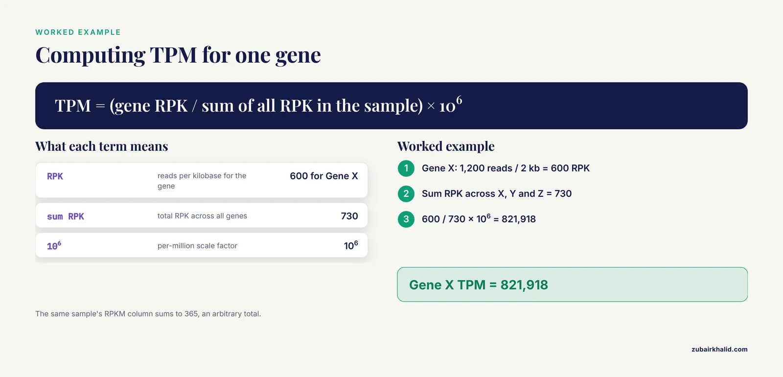
Numbers make this concrete. Consider a toy sample with 2,000,000 mapped reads and three genes.
| Gene | Length (bp) | Reads | RPK (reads per kb) | RPKM | TPM |
|---|---|---|---|---|---|
| Gene X | 2,000 | 1,200 | 600 | 300.0 | 821,918 |
| Gene Y | 500 | 60 | 120 | 60.0 | 164,384 |
| Gene Z | 3,000 | 30 | 10 | 5.0 | 13,699 |
| Sum | 1,290 | 730 | 365.0 | 1,000,001 (rounding) |
RPKM calculation for Gene X: (1,200 × 10^9) / (2,000,000 × 2,000) = 300. TPM calculation for Gene X: 600 / 730 × 10^6 = 821,918. Notice the sums. The RPKM column sums to 365, an arbitrary number that depends on this sample's composition. The TPM column sums to one million by construction.
Now a second sample, sequenced to the same depth, in which composition shifted: Gene X drops to 1,000 reads, Gene Y rises to 900, Gene Z rises to 100.
| Gene | RPK | RPKM | TPM |
|---|---|---|---|
| Gene X | 500 | 250.0 | 214,286 |
| Gene Y | 1,800 | 900.0 | 771,429 |
| Gene Z | 33.3 | 16.7 | 14,286 |
| Sum | 2,333.3 | 1,166.7 | 1,000,001 (rounding) |
Look at what happened. The sum of RPKM values jumped from 365 to 1,166.7 between two samples sequenced at identical depth, because the length and expression composition changed. In sample one, an RPKM of 60 for Gene Y sat in a sample whose RPKM universe totaled 365. In sample two, an RPKM of 900 for Gene Y sat in a universe of 1,166.7. The per-million denominator promised a common scale and did not deliver one. The TPM totals stayed pinned at one million in both samples, so Gene Y's TPM of 164,384 versus 771,429 is a clean statement that its share of the transcript pool changed by roughly 4.7-fold.
Also notice the subtler point. In sample two, Gene X's read count fell only 17 percent while its TPM fell 74 percent. TPM amplifies compositional changes into larger apparent fold changes because it is a strict share of a fixed pool. This is exactly the compositional bias that motivated TMM [1], and it is why neither unit should be fed directly into a statistical test for differential expression.
How to Choose: The Criteria That Decide Real Analyses
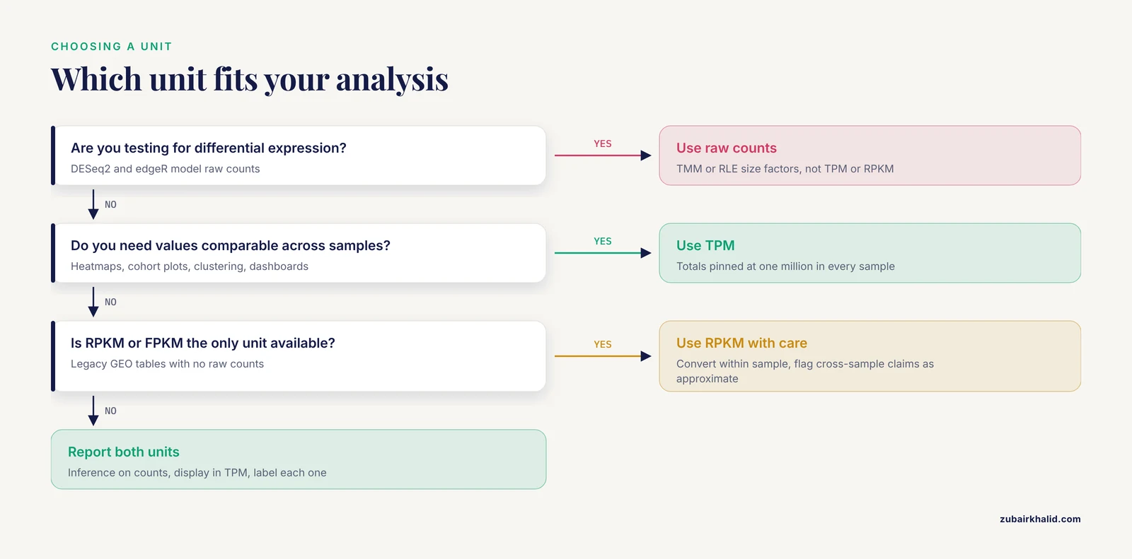
The question "RNA-seq TPM or RPKM" is usually the wrong question, because the right answer for many analyses is a third option. Here is a decision path organized by what you are actually trying to do.
Cross-Sample Comparison of Gene Expression
Use TPM. The fixed sum across samples is the property that makes the comparison valid, and it is the property RPKM lacks. This covers most reporting, visualization, and exploratory analysis: heatmaps, single-gene plots across cohorts, expression atlas entries, and dashboards.
A caveat applies when comparing across species. Gene lengths differ between orthologs in different organisms, and simply length-correcting each species separately does not produce a fair comparison. SCBN addresses this problem directly by formulating a scaling factor for cross-species RNA-seq comparison inside a hypothesis testing framework that accounts for different gene lengths and unmapped genes between species [4]. If your cross-sample comparison is a cross-species comparison, standard TPM is not sufficient on its own.
Within-Sample Comparison of Different Genes
Use TPM. Length correction is mandatory for ranking genes within a sample, and TPM provides it on a scale that is also stable across samples, which costs nothing. RPKM provides the length correction but not the stable scale.
Differential Expression
Use neither TPM nor RPKM as the statistical input. Differential expression methods model raw counts with negative binomial or similar count distributions, and the count structure, including the mean-variance relationship, carries the information the tests need. Convert counts to TPM and you destroy the variance structure the model is built on. The workflow is:
- Quantify at the gene level with a count-based tool such as featureCounts or HTSeq, or at the transcript level with Salmon or kallisto.
- For differential expression, supply raw counts to DESeq2, which uses RLE-style size factors, or edgeR, which uses TMM [1].
- If transcript-level quantifiers were used and gene lengths differ meaningfully between conditions, use the length information as an offset, which is what tximport supports, because count-based size factors alone assume gene lengths are constant across samples. This matters when differential transcript usage or altered isoform usage shifts effective lengths.
The empirical record backs this hierarchy. In the Drosophila benchmark of 726 flies, the normalization method, the distributional assumptions, and the number of biological replicates were the most critical considerations for detecting differential expression, and RPKM was among the failing normalizers [3]. In a comparison of per-sample global scaling and per-gene normalization methods on MAQC and simulated data, methods that combined global scaling with per-gene adjustment achieved slightly higher AUC, specificity above 85 percent, detection power above 92 percent, and actual false discovery rate under 0.06 in the two-replicate MAQC2 setting [5]. And on TCGA laryngeal cancer data, differentially expressed gene lists generated from TPM, FPKM, and DESeq2 normalization did not agree, which led the authors to recommend intersecting DEG lists across normalization techniques before pathway enrichment [6]. The consistent lesson across these studies is that the normalization decision is a first-order scientific decision, not a formatting detail.
Normalizers keep evolving. An adaptive version of TMM that estimates the trimming parameter from the data rather than heuristically, using Jaeckel's estimator with each sample acting as its own reference, showed improved AUC and differential expression performance on SEQC, MAQC2, MAQC3, PICKRELL, and simulated datasets [7]. A Zipf-plot-based method (ZN) avoids assuming that most genes are not differentially expressed, which makes it usable on datasets where the majority of genes are weakly or not expressed, a situation that defeats methods relying on the non-DE majority assumption [8]. None of these are TPM or RPKM, which is the point. The field moved past per-gene-per-million units for inference years ago.
Machine Learning, Networks, and Integrative Models
Here the honest answer is that the best input is often not TPM, and you should benchmark rather than assume. For gene coexpression network construction, a benchmark of 36 workflows found that between-sample normalization had the biggest impact on network quality, and counts adjusted by size factors produced networks that most accurately recapitulated known gene functional relationships [9]. That result pushes against reflexively defaulting to TPM for network work. For genome-scale metabolic modeling, the RLE, TMM, and GeTMM normalizations outperformed TPM and FPKM on model variability [2]. The generalizable finding is that count-based or size-factor-based between-sample normalization tends to preserve signal better than per-gene-per-million units for methods that model relationships among genes, because per-gene-per-million units impose a compositional constraint those methods did not account for.
Legacy Data and Reproducibility
Use the unit the data arrives in, document it exhaustively, and convert with your eyes open. When integrating public datasets, expect batch effects that no choice of TPM versus RPKM will fix. Spike-in-based approaches for removing unwanted variation were evaluated and found insufficiently reliable for standard global-scaling normalization, which motivated RUV, a factor analysis approach on control genes or replicate samples that improved fold-change accuracy and differential expression calls [10]. More recent work refined count-level batch correction, with ComBat-ref preserving counts in a low-dispersion reference batch and adjusting other batches toward it under a negative binomial model, improving sensitivity and specificity over existing methods [11]. The practical takeaway is that choosing TPM over RPKM addresses sample-internal scaling, while batch effects across labs, technicians, and platforms need a separate correction layer, and mixing units from different sources guarantees an uninterpretable result.
Special Sample Types
Sample chemistry changes the calculus. FFPE (formalin-fixed paraffin-embedded) RNA is fragmented and chemically modified, producing count distributions with excessive zeros that standard normalizers handle poorly. SMIXnorm, built on a simplified two-component mixture model with expressed genes modeled by normal distributions and non-expressed genes modeled by zero-inflated Poisson distributions, was developed specifically for FFPE RNA-seq and outperformed general-purpose normalizers at a fraction of the computational cost of its predecessor MIXnorm [12]. If your samples are FFPE, the TPM versus RPKM question is subordinate to choosing a normalizer that models the zero inflation at all.
Worked Scenarios
Scenario 1: Building a Candidate List for qPCR Validation
You ran differential expression with DESeq2 on raw counts, correctly, and now you need to present the validation candidates and sanity-check their behavior. Report log2 fold changes and adjusted p values from the count model. For the figure, plot TPM per gene per sample, because TPM's fixed scale makes the bar chart interpretable and the length correction is already applied. You used two units deliberately, one for inference and one for display, and you labeled both. The mistake to avoid is rerunning the statistics on TPM to make the workflow look uniform. The DEG list you would produce differs by normalization, as demonstrated on TCGA laryngeal cancer data where TPM, FPKM, and DESeq2 each yielded different DEG sets [6], so switching units midstream silently changes your biology.
Scenario 2: Reanalyzing a Published Dataset With Only RPKM Available
You found a 2012 GEO series with FPKM values in the supplemental table and no raw counts. Your options, in order of preference. First, check whether FASTQ or BAM files exist and requantify, which is always preferable. Second, if only FPKM exists, restrict your analyses to within-sample structure and cross-sample comparisons flagged as approximate, convert FPKM to TPM within each sample using the sum relationship, and document the conversion. Third, refuse the temptation to run differential expression tools on the converted values, because the count-level variance information is unrecoverable. State the limitation plainly in your methods section.
Scenario 3: A Coexpression Network Across 40 Tissue Samples
You want gene-gene correlations robust enough to support module detection. The benchmark evidence says the between-sample normalization step dominates the outcome [9], and size-factor-adjusted counts outperformed other preprocessing choices for recapitulating known functional relationships. A defensible pipeline is variance-stabilizing transformation of size-factor-adjusted counts rather than log TPM, with the specific workflow chosen from published benchmarking rather than habit. If you also want to compare your modules against published networks, check what unit the reference used, because scale differences between TPM and size-factor-adjusted counts will shift correlation magnitudes.
Common Mistakes and Limitations
This is the section to reread when something in your pipeline produces a result that looks wrong. Most failures trace to a short list of root causes, and most produce a recognizable error or a silently wrong number. Treat this as a bioinformatics troubleshooting checklist.
- Using TPM or RPKM as the input to differential expression testing. This is the single most common methodological error in published reanalyses. The statistical models in DESeq2 and edgeR expect raw counts. Feeding them TPM changes the mean-variance relationship, inflates apparent significance, and produces DEG lists that disagree with count-based analysis [6].
- Mixing units from different sources. Joining a TPM matrix from one study with an RPKM matrix from another, or TPM from one pipeline with TPM from another computed with different annotations, produces columns on different scales. Symptom: a PCA plot where samples separate by source dataset rather than biology, or correlation heatmaps with a block structure that matches study origin exactly.
- Annotation version mismatch. Gene lengths come from a GTF or GFF file, and changing annotation releases changes transcript definitions and lengths, especially at untranslated regions. A matrix of TPM computed against GENCODE release 19 is not directly comparable to one computed against release 44 for the same genome. Symptom: the same sample reprocessed with a new annotation shows systematically shifted TPM for a subset of genes. Fix: recompute all values from counts with a single annotation, and record the release in your methods.
- Dividing by the wrong denominator. RPKM and FPKM should use mapped reads or fragments, not raw reads including those that failed alignment. Symptom: all values slightly deflated relative to a collaborator's, with the ratio equal to the mapping rate. Also watch for deduplicated counts used as the numerator against a non-deduplicated library size, or the reverse, which distorts values non-uniformly.
- Wrong length units. Gene lengths must enter the formula in the units the formula expects, and off-by-1000 errors here divide every value by a constant, which some plots tolerate and every absolute statement destroys. Symptom: a colleague's TPM values are exactly 1000-fold different from yours. This is the rare silent error that announces itself.
- Sum of TPM is not one million. If you filter low-expression genes after computing TPM, the remaining values no longer sum to one million, and downstream methods that assume the fixed sum will misbehave. Symptom: colSums on your TPM matrix returns values like 840,000. Fix: either accept it and document it, or filter on counts first and recompute TPM on the retained genes.
- Applying length normalization to tag-based or 3'-end counting protocols. Methods that count reads near the 3' end effectively count molecules, not length-dependent coverage, so dividing by gene length introduces bias in the opposite direction of the one you are correcting. For such protocols, gene-length correction is inappropriate, and count-based normalization or UMI-aware handling is the correct path.
- Assuming normalization handles batch effects. It does not. TMM, RLE, TPM, and RPKM adjust for depth and composition, not for library preparation chemistry, lab, or platform. Spike-in-based correction proved unreliable for standard global scaling, and factor-analysis approaches such as RUV were developed because usual normalization accounts for sequencing depth while failing to correct more complex unwanted technical effects [10]. Negative-binomial batch correction layered on top, in the spirit of ComBat-ref, addresses the residual structure [11]. Plan for both steps, not one.
- Ignoring zero inflation in low-input or FFPE samples. When a large fraction of genes are weakly or not expressed, normalizers that assume a non-DE majority or a well-behaved central mass lose their anchor. Methods built for this regime, such as ZN and SMIXnorm for FFPE [12], exist for a reason.
- Cross-species comparisons with plain TPM. Orthologs have different lengths and species have different gene complements, so per-species TPM is not a fair comparison scale. Use a method that models the problem, such as SCBN [4], rather than eyeballing TPM heatmaps across species.
- Double-counting paired-end fragments as reads. Summing both mates inflates counts for longer insert libraries. Use fragment-level counts from the aligner or quantifier, which is the entire reason FPKM exists.
- Trusting a single normalization. Given that DEG lists, network topologies, and metabolic model contents all shift with normalization choice [2][9][6], running your key analysis under two normalizations and reporting the intersection is cheap insurance, not statistical weakness.
The broader limitation to state once: TPM and RPKM are relative measures inside a compositional system, so neither can report absolute transcript abundance, and any analysis question that depends on absolute RNA quantity per cell or per tissue mass needs different data, such as spike-in-calibrated or RNA-content-corrected measurements.
Frequently Asked Questions
Is TPM better than RPKM?
Yes, for cross-sample gene-level comparisons, because TPM values sum to one million in every sample while RPKM sums drift with sample composition. RPKM remains useful only for reading legacy data.
What is the actual difference between RNA-seq TPM and RPKM?
Both correct for gene length. TPM then rescales by the sum of length-corrected counts within the sample, fixing the total at one million. RPKM rescales by the raw library size, leaving sample totals free to vary.
Can I convert RPKM to TPM?
Within one sample, yes. Divide each gene's RPKM by the sum of all RPKM values in that sample and multiply by one million. This requires the full gene set and consistent gene lengths, and it fixes only within-sample structure, not cross-sample comparability.
Should I use TPM for differential expression analysis?
No. Differential expression methods such as DESeq2 and edgeR model raw counts with count-based distributions and require the count variance structure. Use raw counts with TMM or RLE size factors, and report TPM only for figures.
When should I use RPKM instead of TPM?
Practically never for new analyses. Use FPKM or RPKM values when integrating with legacy datasets where they are the only available unit, and use FPKM rather than RPKM when working with paired-end fragment counts.
Do TPM values always sum to one million?
Only across all genes as originally computed. Filtering genes after computing TPM lowers the sum, so check colSums on your matrix and either filter before computing TPM or document the deviation.
Sources
- A scaling normalization method for differential expression analysis of RNA-seq data
- A benchmark of RNA-seq data normalization methods for transcriptome mapping on human genome-scale metabolic networks
- Comparison of normalization and differential expression analyses using RNA-Seq data from 726 individual Drosophila melanogaster
- A statistical normalization method and differential expression analysis for RNA-seq data between different species
- A comparison of per sample global scaling and per gene normalization methods for differential expression analysis of RNA-seq data
- Differentially expressed genes of RNA-seq data are suggested on the intersections of normalization techniques
- Normalization of RNA-Seq data using adaptive trimmed mean with multi-reference
- A Zipf-plot based normalization method for high-throughput RNA-seq data
- Robust normalization and transformation techniques for constructing gene coexpression networks from RNA-seq data
- Normalization of RNA-seq data using factor analysis of control genes or samples
- Highly effective batch effect correction method for RNA-seq count data
- SMIXnorm: Fast and Accurate RNA-Seq Data Normalization for Formalin-Fixed Paraffin-Embedded Samples