Writing a Bioinformatics Manuscript with R Markdown
By Dr. Zubair Khalid, DVM, MS, PhD ·

By the end of this guide you will be able to build a complete bioinformatics manuscript as a single R Markdown document: a file that mixes your methods text, your R for bioinformatics code, your figures, your tables, and your statistics, all generated from one reproducible source. You will install the right tools, write a proper YAML header, load Bioconductor packages in a controlled setup chunk, run a differential expression analysis inline, produce journal-resolution figures with captions and cross-references, manage a bibliography, render the document to PDF and HTML, and fix the errors that stop most people on their first attempt.
R Markdown is a literate programming format. Literate programming means prose and executable code live in the same file, and the code runs every time the document is rebuilt. For a bioinformatics manuscript this matters because the Results section is only trustworthy if the numbers in it come from the same code that produced the figures. Reviews of bioinformatics practice repeatedly identify reproducibility as the central weakness of published computational analyses, and teams building large collaborative pipelines, such as the H3ABioNet network across 17 African countries, treat portable and reproducible workflows as a first-class deliverable rather than an afterthought [1]. R Markdown is one of the simplest tools that puts that principle inside the manuscript itself.
Why R Markdown Suits a Bioinformatics Manuscript
A conventional manuscript is written in Word, the analysis lives in a dozen scripts scattered across directories, the figures were exported weeks ago, and nobody, including the author, can regenerate Figure 3 from the raw count matrix. R Markdown inverts this. The manuscript document is the analysis. When a reviewer asks for an additional panel, you edit one chunk, re-render, and every downstream number, p-value, and figure updates consistently.
Two properties make this practical. First, R for bioinformatics has mature scientific packages: Bioconductor, the open-source project that curates genomics software for R, provides versioned, peer-reviewed packages for RNA-seq, methylation, single-cell, and nearly every other assay type. Second, knitr, the engine that executes chunks inside R Markdown, records session information and supports caching, so a 40-page methods section can re-render without recomputing everything.
There is also a cost to not doing this. Workflow researchers describe "workflow decay," the situation where a pipeline stops working after a few years because it depended on a specific, undocumented computing platform [2]. A manuscript whose analysis is embedded and version-controlled decays far more slowly than one whose analysis lives only in a departed postdoc's home directory. Published computational pipelines increasingly adopt this style. The GCAC virtual-screening system, for example, combines R statistical packages with literate programming tools inside a workflow environment so that every model-building step is traceable [3]. Targeted methylation sequencing protocols now explicitly require a structured downstream stage in R, with methylKit for differential methylation, PCA, and regional profiling, all embedded in a unified reproducible pipeline with explicit reporting of intermediate outputs [4]. An rmarkdown bioinformatics manuscript is the document-level expression of the same idea.
R Markdown is not the only tool for this. Later in this article I cover when a project outgrows it. For a paper, a thesis chapter, or a collaborative report, it remains the fastest path from data to a submission-ready PDF.
What You Need Before You Start
Install the following before writing a single sentence.
- R (version 4.2 or newer recommended). Download from CRAN at cran.r-project.org.
- RStudio Desktop, the integrated development environment that renders R Markdown with one click. Download from posit.co.
- Pandoc, the universal document converter that turns rendered Markdown into PDF, Word, and HTML. RStudio bundles a copy, so you usually do not install it separately.
- LaTeX, needed only if you want PDF output. The lightest option is the tinytex package, which installs a minimal distribution and adds packages on demand.
- Bioconductor and the packages your analysis uses.
Run this in the R console:
install.packages(c("rmarkdown", "knitr", "tinytex", "renv", "bookdown"))
tinytex::install_tinytex()

if (!require("BiocManager", quietly = TRUE)) {
  install.packages("BiocManager")
}
BiocManager::install(c("DESeq2", "BiocStyle", "EnhancedVolcano", "apeglm"))
Verify the installation:
packageVersion("rmarkdown")
packageVersion("DESeq2")
Expected output in a 2024-era environment:
[1] '2.25.7'
[1] '1.44.0'
Your version numbers will differ. Write them down, because a Bioconductor tutorial or manuscript is only reproducible against specific versions.
Step 1: Set Up the Manuscript Project
Create a self-contained project directory. Everything the manuscript needs, data, scripts, bibliography, rendered output, lives inside it.
manuscript/
├── manuscript.Rmd
├── references.bib
├── data/
│   ├── counts.tsv
│   └── sample_meta.tsv
├── results/          (generated intermediates)
├── figures/          (generated figures)
└── renv/             (package lockfile, optional but recommended)
Open this folder as an RStudio Project (File, New Project, Existing Directory). Using a Project guarantees the working directory is the project root, which makes relative paths such as data/counts.tsv work on your laptop and on a collaborator's machine.
If you want frozen package versions, initialize renv, which snapshots every package and version into a lockfile:
renv::init()
renv::snapshot()
Reviewers and co-authors can then run renv::restore() and get your exact package library.
Step 2: Write the YAML Header
The YAML header is the metadata block at the top of the file, delimited by three hyphens. It controls the title, authors, output format, and bibliography. For a bioinformatics manuscript rendered through Bioconductor's style package, a solid starting point is:
---
title: "Transcriptomic response of hepatocytes to compound X"
author:
  - name: "First Author"
    affiliation: "Department of Biology, Example University"
    email: "[email protected]"
  - name: "Second Author"
    affiliation: "Institute of Genomics, Example University"
date: "`r Sys.Date()`"
output:
  bookdown::pdf_document2:
    toc: false
    number_sections: true
  bookdown::html_document2:
    toc: true
    toc_float: true
bibliography: references.bib
link-citations: true
geometry: margin=1in
fontsize: 11pt
---
Each parameter matters:
- output controls the rendered format.
bookdown::pdf_document2andbookdown::html_document2are the bookdown variants of the standard outputs, and they activate automatic numbering of figures and tables plus cross-references with\@ref(). If you do not need numbered sections, plainpdf_documentworks and pulls in fewer dependencies. - bibliography points to a BibTeX file. R Markdown resolves in-text citations against it automatically.
- link-citations makes citations clickable in HTML output, which reviewers appreciate.
- fontsize and geometry handle common journal formatting without a separate LaTeX template.
- date is wrapped in backticks and
r Sys.Date(), which is inline R code. It stamps the render date so re-prints are distinguishable.
For journals that accept LaTeX submissions, the rticles package provides publisher-specific templates (Elsevier, Springer, PLOS and others) that drop into the same output: field.
Step 3: Create the Setup Chunk
Every R Markdown document should start with a chunk named setup. A chunk is a fenced block of R code that knitr evaluates during rendering. Place this immediately after the YAML header:
knitr::opts_chunk$set(
  echo = FALSE,
  warning = FALSE,
  message = FALSE,
  fig.width = 6,
  fig.height = 4,
  dpi = 300
)
set.seed(2026)
What each option does:
- echo = FALSE hides code in the final manuscript. In a Results section you usually show figures and numbers, not code. In a Methods or tutorial-style document, set
echo = TRUEglobally instead. - warning = FALSE, message = FALSE suppress package startup text and deprecation notices from the rendered output. Hide them deliberately, not accidentally.
- fig.width, fig.height, dpi control figure dimensions and resolution. A dpi of 300 meets the raster-image requirement of most journals.
- set.seed(2026) fixes the random number generator so any stochastic step, PCA subsampling, random forest, bootstrap, produces identical output on every render.
The chunk option include=FALSE in the header line means the chunk runs but its output is not printed. This is standard for setup.
Step 4: Load Packages and Data, and Record Provenance
Load Bioconductor packages in their own chunk, early, so conflicts surface before analysis code:
library(DESeq2)
library(EnhancedVolcano)
library(ggplot2)
Then read the data. Keep raw data out of git if it is large or restricted, and record exactly where it came from in the text:
counts <- read.delim("data/counts.tsv", row.names = 1)
meta   <- read.delim("data/sample_meta.tsv")
meta$condition <- factor(meta$condition, levels = c("control", "treated"))
stopifnot(identical(colnames(counts), meta$sample_id))
The stopifnot() line is a cheap guard. If column names in the count matrix do not match sample identifiers in the metadata, rendering stops immediately with an informative error instead of producing a beautifully formatted manuscript built on silently misaligned samples.
Finish the setup with a provenance chunk that prints itself into the rendered document:
sessionInfo()sessionInfo() prints the R version, operating system, and every attached package with its version. Many journals now request it, and it is the single cheapest reproducibility investment you can make. Packages such as MeTime, built for longitudinal metabolomics, retain intermediate results and provenance inside a central container precisely so that automatically generated HTML and PDF reports remain auditable, and the same principle applies at manuscript scale [5].
Step 5: Run the Analysis in Chunks
Now the Results section. Here is a minimal differential expression analysis with DESeq2, the Bioconductor workhorse for RNA-seq count data. Each chunk should do one logical thing and print one result.
dds <- DESeqDataSetFromMatrix(
  countData = round(as.matrix(counts)),
  colData   = meta,
  design    = ~ condition
)
dds <- DESeq(dds)
res <- results(dds, contrast = c("condition", "treated", "control"))
res_df <- as.data.frame(res[order(res$padj), ])
With cache=TRUE, knitr stores the chunk's results on disk and skips re-execution on later renders unless the chunk code changes. For a chunk that calls DESeq(), which fits negative binomial models and can take minutes to hours, this turns a 20-minute re-render into a 5-second one.
Show the reader a summary, not the full table:
knitr::kable(
  head(res_df[, c("baseMean", "log2FoldChange", "padj")], 5),
  digits = 2,
  caption = "Most significant differentially expressed genes (treated vs control)."
)
Expected output in the rendered PDF:
| baseMean | log2FoldChange | padj | |
|---|---|---|---|
| GENE_A | 482.1 | 2.41 | 3.2e-08 |
| GENE_B | 156.7 | -1.98 | 5.9e-07 |
| GENE_C | 903.4 | 1.76 | 1.1e-06 |
Because the table is generated by code, the padj values in your manuscript are guaranteed to match the res object, which generated your figures, which match your statistics. That consistency is the whole point of the format.
In the prose around the chunk, you can reference computed values directly so text and results never drift apart:
n_sig <- sum(res_df$padj < 0.01, na.rm = TRUE)Treatment with compound X altered r n_sig genes at an adjusted p-value below 0.01.
If n_sig is 214, the sentence reads "Treatment with compound X altered 214 genes at an adjusted p-value below 0.01." Change the analysis and the sentence updates on the next render.
Step 6: Figures With Captions and Cross-References
Figures belong in chunks with a caption. Using the bookdown output formats from Step 2, you get automatic numbering:
EnhancedVolcano::EnhancedVolcano(
  res_df,
  x = "log2FoldChange",
  y = "padj",
  lab = rownames(res_df),
  pCutoff = 1e-2,
  FCcutoff = 1,
  title = NULL,
  subtitle = NULL
)
In the text, reference the figure with:
Differential expression is summarized in Figure
\@ref(fig:volcano).
This renders as "Figure 1." Rename the chunk or delete it, and the reference updates or fails loudly during rendering. A silent "see Figure 3" pointing at the wrong panel is one of the most common reviewer complaints, and this mechanism eliminates the entire class of error.
Step 7: Citations and the Bibliography
Store references in a BibTeX file, references.bib, in the project root:
@article{love2014,
  title   = {Moderated estimation of fold change and dispersion for RNA-seq data with DESeq2},
  author  = {Love, Michael I and Huber, Wolfgang and Anders, Simon},
  journal = {Genome Biology},
  volume  = {15},
  number  = {12},
  pages   = {550},
  year    = {2014}
}
Cite in the text with square brackets and an at-sign:
Differential expression was tested with DESeq2 [@love2014].
R Markdown converts this to "Differential expression was tested with DESeq2 (Love et al. 2014)" and builds the reference list at the end of the document. The rendered citations match the bibliography automatically, so the days of a reference list numbered differently from the in-text citations are over. Export entries directly from PubMed or Zotero to avoid transcription errors, which are themselves a reproducibility defect.
Step 8: Render the Manuscript
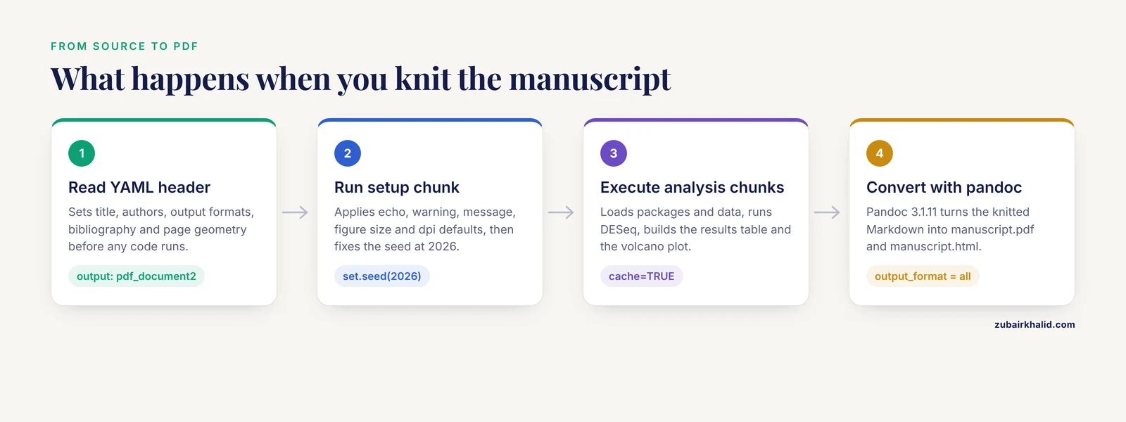
Render from the console, or press the Knit button in RStudio:
rmarkdown::render("manuscript.Rmd", output_format = "all")Expected console output:
processing file: manuscript.Rmd
  |.....                                    |  12%
  ordinary text without R code
  |..........                               |  25%
label: setup (with options)
...
output file: manuscript.knit.md
pandoc 3.1.11 -> manuscript.pdf
pandoc 3.1.11 -> manuscript.html
The finished manuscript.pdf and manuscript.html appear in the project root. Render with output_format = "all" before submission so you catch formatting problems in both formats. To produce the Word file many co-authors and journals still request, add bookdown::word_document2 to the YAML output list.
Key Options at a Glance
| Option | Where | What it controls | Typical manuscript value |
|---|---|---|---|
echo | chunk | Whether code is printed | FALSE in Results, TRUE in Methods tutorials |
eval | chunk | Whether code runs | TRUE, set FALSE for illustrative snippets |
cache | chunk | Skips re-execution if code unchanged | TRUE for slow chunks (alignment, model fitting) |
fig.cap | chunk | Figure caption, enables numbering | Descriptive sentence per figure |
dpi | chunk | Raster resolution | 300 for journal figures |
out.width | chunk | Displayed width in output | "90%" or "3in" |
results | chunk | How textual output is treated | 'asis' when emitting raw Markdown tables |
include | chunk | Runs code but hides it and its output | FALSE for data loading |
output: | YAML | Rendered formats | bookdown::pdf_document2 plus HTML |
bibliography | YAML | BibTeX file used for citations | references.bib |
link-citations | YAML | Clickable citations in HTML | true |
cache.path | chunk | Directory for cached chunk output | "results/cache/" |
Common Errors and Their Exact Fixes
"pandoc version 1.12.3 or higher is required and was not found (see the help page ?rmarkdown::pandoc_version) for details." RStudio cannot find a recent pandoc. Update RStudio, which bundles pandoc, or install pandoc separately and confirm it is on your system PATH.
"! LaTeX Error: File \inconsolata.sty' not found." The minimal tinytex distribution lacks a LaTeX package the template needs. Run tinytex::tlmgr_install("inconsolata")`, or install the missing package named in the error. Alternatively, drop the font or geometry requirement from the YAML header.
"Error: package or namespace load failed ... there is no package called 'BiocStyle'." A Bioconductor package was never installed on the machine doing the rendering. Run BiocManager::install("BiocStyle"). This error most often appears when a collaborator or continuous integration system renders the document without your package library, which is exactly what the renv lockfile from Step 1 prevents.
"Error in eval(expr, envir, enclos): object 'dds' not found." The chunk referencing dds ran without its dependency, almost always because you cleared the cache or renamed a chunk while a later chunk still depended on it. knitr's cache is per-chunk, not global: if chunk A is cached and chunk B is not, editing the data changes nothing downstream unless you also clear A. Fix with knitr::clean_cache() and re-render, and keep cache dependencies explicit by chaining chunk names in the dependson option.
"Error in DESeqDataSetFromMatrix(countData = ..., colData = ..., design = ...): some variables in design formula are characters or factors not present in colData." The design formula references a column name that does not exist in the metadata, typically because of a typo or because the metadata lost its row names. Print colnames(meta) in a scratch chunk and reconcile.
A figure renders blank or at tiny size in PDF. Usually fig.height and fig.width are unset and the default of 7 by 5 inches is squeezed by the page, or the plot was created before a ggplot2 layer was added. Set dimensions explicitly in the chunk header, as in Step 6.
Checking That the Manuscript Is Correct
Verification is a habit, not a one-time check.
- Delete all caches and render from scratch. Run
knitr::clean_cache()followed byrmarkdown::render("manuscript.Rmd"). If the document renders cleanly and the numbers in the abstract still match, your cache was not hiding broken dependencies. - Render on a second machine or account. The strongest check available locally. Any hard-coded path such as
/home/you/datawill fail here, and that failure is a gift, because a reviewer or reader would have found it later. - Cross-check three numbers manually. Pick one padj value, one figure label, and one in-text inline value such as the gene count above, and confirm they match between the rendered PDF and the R objects.
- Confirm the session information block is current. It should list the packages you actually used, with plausible versions, rendered on the render date.
- Read the diff after a re-render. If a sentence about fold changes changed when you did not touch the analysis, something upstream moved, and you want to know before submission rather than after publication.
Common Mistakes and Limitations
The most frequent failures in an rmarkdown bioinformatics manuscript, and how to avoid them:
- Caching everything blindly. Cached chunks do not re-run, so an upstream data change propagates silently nowhere. Cache only genuinely slow chunks, and set
dependsonor clear the cache whenever inputs change. - Never recording the session. A manuscript without
sessionInfo()output is not reproducible in any meaningful sense. Two DESeq2 major versions can differ in default behaviors, and readers need to know which one produced your numbers. - Hiding all code, everywhere. Setting
echo=FALSEglobally makes the document pretty and unauditable. At minimum, keep a Methods appendix withecho=TRUEchunks showing parameter choices, filtering thresholds, and model formulas. - Running hours of compute inside the manuscript. If a step takes six hours on a cluster, it does not belong in a render. Write the expensive step as a standalone script, run it separately, and have the manuscript read its output. Reviews of pipeline practice are explicit that scripting languages and notebooks, R included, are sufficient for small-scale single-user analysis but that large-scale, shareable, maintainable pipelines belong in scientific workflow systems [6]. A published TCGA regulatory-network workflow made this split deliberately: Nextflow handled downloading, preprocessing, and orchestration, while a companion R package held the data-management and filtering functions the analysis relied on [7].
- Hard-coded absolute paths.
read.delim("/Users/you/secret_project/counts.tsv")breaks the moment the project moves. Relative paths from the project root, as used throughout this guide, survive collaboration. - Skipping
set.seed(). Any stochastic step renders differently each time, and a reviewer who re-runs your document will get different gene counts than the ones in your abstract. - Treating the rendered output as the archive. The PDF is a snapshot. The archive is the project directory: Rmd, data, bib, lockfile, and rendered output, in version control.
- Overstating what the format delivers. R Markdown guarantees that the code shown produced the output shown. It does not guarantee the code is correct, the statistics are appropriate, or the data were generated properly. Those remain your scientific judgment.
A practical tip set that survives every project: render early and often rather than once at the end, keep one chunk per logical result, name chunks after their content (deseq, volcano) rather than their order (chunk14), and commit the rendered files alongside the source so co-authors can see changes without re-rendering.
Scaling Up: When a Manuscript Is Not Enough
R Markdown is a manuscript-scale tool. When an analysis must run routinely across many samples, many compute environments, or many studies, move the heavy processing into a workflow system and keep the R Markdown document as the reporting layer. This layered design is now standard in the field. H3ABioNet built portable, reproducible workflows for variant calling, 16S analysis, genotyping, and SNP imputation precisely because scalable reproducibility on heterogeneous computing environments requires infrastructure beyond a single script [1]. Reviews of scientific workflow systems map the requirements, modularity, reusability, cluster support, that push projects from notebooks toward systems such as Nextflow and Snakemake [6]. Even in model-driven disciplines such as quantitative systems pharmacology, groups formalize the model-building workflow itself so that each iterative application is documented and qualified rather than improvised [8]. The pattern to aim for: a versioned pipeline produces the count matrices and intermediate tables, and the R Markdown manuscript consumes those outputs, performs statistics and visualization, and generates the submission-ready document with every number traceable to code.
Frequently Asked Questions
Do I need to show all my code in the manuscript?
No, but you need it in the project. Most papers set echo=FALSE in Results and include a supplementary document or Methods appendix with code visible. The rendered PDF should read as a paper, the repository should read as an analysis.
Can I submit an R Markdown manuscript directly to a journal?
Usually you submit the rendered PDF or Word file, plus the Rmd and data as supplementary material or a repository link. The rticles package provides publisher-formatted templates that produce submission-compliant PDFs from the same source file.
How do I handle analysis steps that run on a cluster?
Keep them outside the manuscript. Run the alignment or model fitting as a standalone script or within a workflow engine, save the outputs to the project directory, and have the manuscript load those files. This mirrors published pipeline designs that separate preprocessing stages from the downstream R analysis stage [4].
What is the difference between R Markdown and Quarto?
Quarto is the successor publishing system from the same team, with a different engine and broader language support. Existing R Markdown skills transfer almost completely, and R Markdown remains fully supported, so either is a sound choice for a manuscript today.
How do I make figures meet journal resolution requirements?
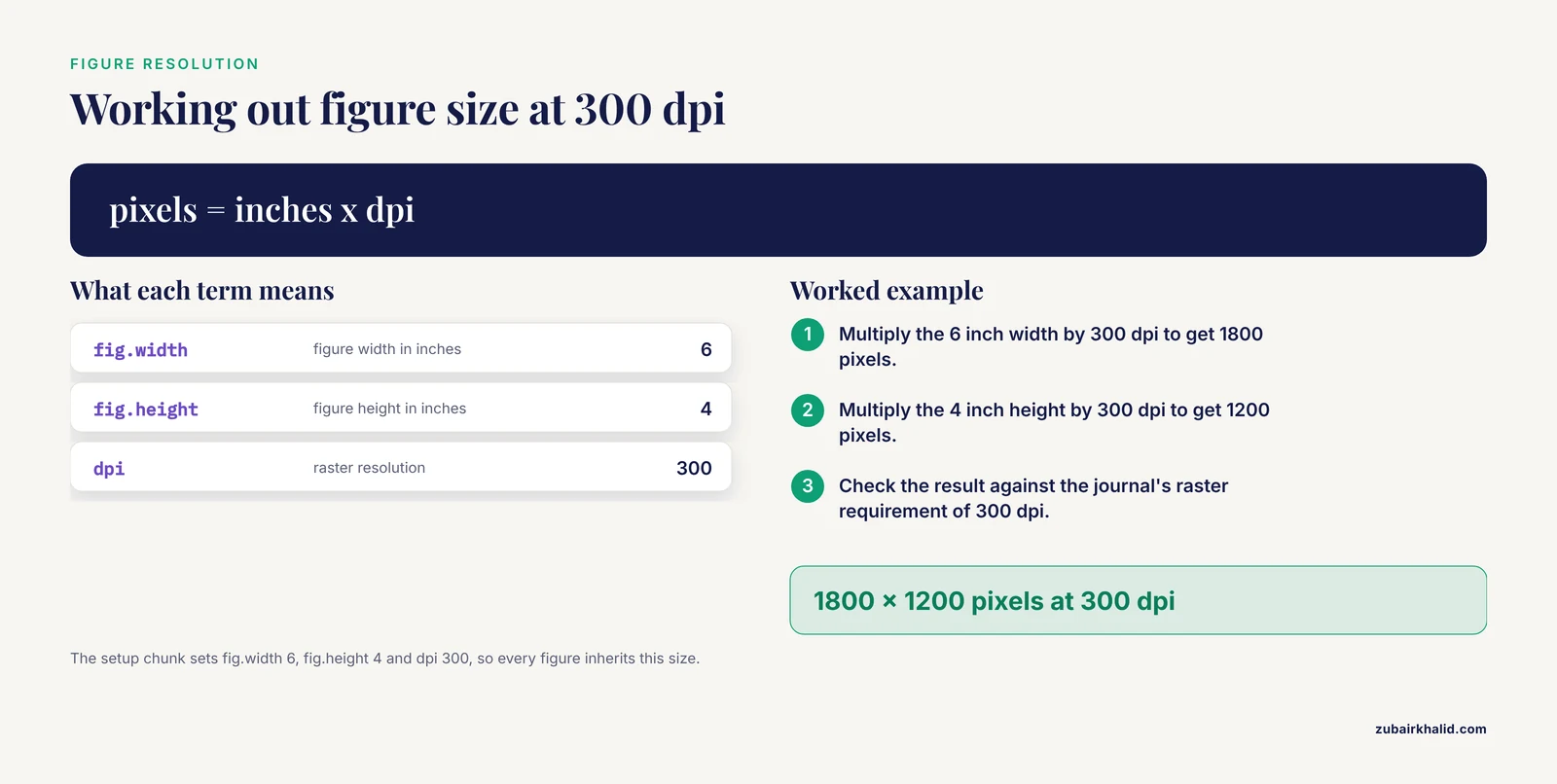
Set dpi=300 in the chunk options for raster figures, or save ggplot objects with ggsave() and the device set to PDF or SVG for vector output. Check the target journal's figure guidelines for exact dimensions before finalizing.
How do I keep package versions stable across co-authors' machines?
Use renv. Initialize it in the project, snapshot the library, and commit renv.lock to version control. Co-authors run renv::restore() and receive the exact package versions your results were produced with.
How do I share the reproducible analysis with reviewers?
Publish the project directory as a GitHub or Zenodo repository with a DOI, containing the Rmd, bibliography, small data files or download instructions, and the lockfile. State in the Data Availability section how to render the document from scratch.
Does R Markdown replace a proper bioinformatics pipeline?
No. It replaces the disconnected analysis scripts behind a manuscript. Once an analysis must run repeatedly, at scale, or across computing environments, scientific workflow systems provide the modularity and maintainability that manuscripts and notebooks cannot [6]. The strongest setups use both, a pipeline for computation and an R Markdown document for reporting.
Sources
- Developing reproducible bioinformatics analysis workflows for heterogeneous computing environments to support African genomics.
- An evolving computational platform for biological mass spectrometry: workflows, statistics and data mining with MASSyPup64.
- GCAC: galaxy workflow system for predictive model building for virtual screening.
- A Guide to Enzymatic Targeted Methylation Sequencing Bioinformatics Workflow: Best Practices.
- MeTime: an R package for reproducible longitudinal metabolomics data analysis.
- Developing and reusing bioinformatics data analysis pipelines using scientific workflow systems.
- Reproducible processing of TCGA regulatory networks.
- Quantitative Systems Pharmacology: An Exemplar Model-Building Workflow With Applications in Cardiovascular, Metabolic, and Oncology Drug Development.