Building a Reproducible Genomic Analysis Pipeline with pandas
By Dr. Zubair Khalid, DVM, MS, PhD ·

By the end of this article you will be able to build a reproducible genomic analysis pipeline with pandas that reads variant data, computes per-sample allele frequencies, aggregates them into a position-aligned matrix, and writes versioned outputs that another person can rerun on a different machine and get identical numbers. You will also learn how to structure the project as a reusable template, how to verify each intermediate result, and how to diagnose the pandas errors that show up most often in genomic work.
Here is what you need installed or on hand before you start:
- Python 3.10 or newer
- pandas 2.x, NumPy, and PyArrow (for parquet output)
- Biopython, if your workflow touches FASTA, GenBank, or other biological formats
- A conda or mamba installation for environment management, or a comfort with virtualenv plus a pinned requirements file
- A small set of real input files. A mitochondrial VCF from your own cohort works well, and any standard VCF with an AD (allelic depth) field will let you follow the worked example end to end
- Roughly 30 minutes for the walkthrough and another 30 for wiring the reproducibility scaffolding
Why pandas Belongs in a Genomic Analysis Pipeline
Genomic analysis pipelines usually have two halves. The first half is compute-heavy alignment and variant calling, handled by tools like BWA, GATK, or bcftools. The second half is data wrangling: filtering variant tables, joining sample metadata, computing per-sample statistics, and reshaping results into matrices for plotting and cohort comparison. That second half is where pandas is strongest, and it is also where most non-reproducibility creeps in, because analysts tend to do it interactively in notebooks and never freeze the logic.
Reproducibility here means something concrete. Given the same inputs, your pipeline produces byte-identical (or at least numerically identical) outputs on a different date, on a different machine, run by a different person. That requires four things: a pinned environment, deterministic code, fixed input formats, and an ordered execution path with no hidden manual steps.
A published example of this design in the genomics literature is Mito_Plot, an open-source pipeline for quantifying and visualizing mitochondrial DNA heteroplasmy. Mito_Plot accepts standard mitochondrial VCF files, calculates the Mutant Allele Frequency (MAF) from allelic depth information, and aggregates MAF values from multiple samples into a unified matrix aligned by genomic position so that cross-sample comparison becomes a direct tabular operation [1]. The authors specifically built it because existing tools focused on single-sample visualization or required substantial manual preprocessing, which limited scalability to large cohorts [1]. That design decision, standardized input in, standardized matrix out, is exactly the pattern you will implement in this article with pandas, and you can extend it to any variant-level or feature-level genomic data.
Two clarifications before the code. First, pandas is not a variant caller and should not be asked to parse raw BAM files. Feed pandas tidy tabular data, typically extracted from VCF, GFF, or expression matrices. Second, python for bioinformatics does not mean replacing established command-line tools. It means wrapping them in deterministic glue code so the whole workflow can be rerun with one command.
The Reproducibility Contract
Before writing any analysis code, define the contract your pipeline must satisfy. Write it at the top of your README as a checklist:
- Environment: every dependency version is pinned and recorded.
- Inputs: every input file has a declared format, a checksum, and a documented source.
- Determinism: every stochastic step has a fixed seed, and no step depends on dictionary iteration order, file listing order, or floating-point accumulation order across threads.
- Statelessness: running the pipeline twice in a clean directory produces identical outputs. No step mutates its own inputs.
- Traceability: every output file records the git commit, the input checksums, and the software versions that produced it.
If any of the five fails, you do not have a reproducible pipeline yet, regardless of how good the analysis is.
Step 1: Pin the Environment
Use conda with an explicit export, or pip with a fully pinned requirements file. The critical rule is that the file that pins versions is itself version controlled.
Create the environment:
conda create -n genv python=3.11 pandas numpy pyarrow biopython -y
conda activate genv
pip freeze > requirements.txt
git add requirements.txt
For tighter control, prefer an exported environment file, which records build strings for conda packages:
conda env export --no-builds > environment.ymlThen record Python and library versions inside your pipeline itself, so every output carries its own provenance:
import sys, platform
import pandas as pd
import numpy as np
import bio  # biopython

def write_provenance(outdir):
    versions = {
        "python": sys.version.split(),
        "platform": platform.platform(),
        "pandas": pd.__version__,
        "numpy": np.__version__,
    }
    with open(f"{outdir}/provenance.json", "w") as f:
        import json
        json.dump(versions, f, indent=2)
A common failure here is a pipeline that works with pandas 1.5 and silently changes behavior under pandas 2.x, most often around integer NA handling and copy-on-write semantics. Pinning is not bureaucratic decoration. It is the difference between a result and a rumor.
Step 2: Lay Out the Project as a Template
A reproducible genomic analysis pipeline needs a fixed directory format so that a collaborator can find every artifact without asking you. This layout is the template I use, and it works unchanged across RNA-seq, variant, and metadata projects:
project/
  README.md
  environment.yml
  config.yaml          # parameters, sample sheet path, thresholds
  data/
    raw/               # never modified, checksums recorded
    metadata/          # sample sheet CSV, phenotypes
  src/
    01_parse_vcf.py
    02_filter_variants.py
    03_maf_matrix.py
    04_plots.py
  results/
    intermediate/
    final/
  logs/
  tests/
    test_maf.py
Three rules make this template work. Numbered scripts encode execution order explicitly rather than implicitly. The data/raw directory is read-only in practice, and any script that writes into it is wrong. And every tunable parameter, such as a quality threshold or a minimum depth, lives in config.yaml, never hardcoded in src/. A collaborator reruns your pipeline by editing one YAML file, not by hunting through four scripts for magic numbers.
Step 3: Define the Input Format Contract
Decide and document your input format before writing the parser. For the worked example that follows, the input is a set of VCF files, one per sample, each containing variant records with a POS column and an AD field holding allelic depths (the read counts supporting each allele at that position).
Write the contract into the README:
- One VCF per sample, uncompressed or bgzipped
- Sample ID encoded in the filename as
SAMPLE.vcf - The AD field must be present in INFO or FORMAT. If your caller emits DP only, the pipeline will fail loudly at step 01, which is the desired behavior
Formalizing the format sounds pedantic until the day a collaborator hands you files where the AD field is missing for indels. A declared contract plus a loud failure at parse time beats a silent NaN three steps downstream every time.
This is also where Biopython earns its place. If your workflow reads FASTA or GenBank reference files, Biopython's SeqIO gives you a stable, documented API for them. For a biopython tutorial level summary, the two patterns you need most are:
from Bio import SeqIO

# Read a reference genome or mitochondrion FASTA
for record in SeqIO.parse("chrM.fasta", "fasta"):
    print(record.id, len(record.seq))

# Fetch a subsequence around a variant position
record = next(SeqIO.parse("chrM.fasta", "fasta"))
context = record.seq[3242:3270]  # 0-based half-open interval
print(context)
Note the 0-based half-open interval convention. VCF positions are 1-based. Every off-by-one bug in genomic pandas code traces back to mixing these two conventions, so convert once, at the boundary, and work in 0-based pandas coordinates everywhere else.
Step 4: Parse VCF Records into a pandas DataFrame
The following is a complete, runnable script. It uses the VCF text itself, which is a structured, tab-separated format, and extracts the fields pandas needs.
# src/01_parse_vcf.py
"""
Parse one VCF per sample into a tidy per-sample variant table.
Input contract: data/raw/SAMPLE.vcf with an AD field.
Output: results/intermediate/variants_SAMPLE.parquet
"""
import argparse
from pathlib import Path
import pandas as pd

def parse_one_vcf(path: Path) -> pd.DataFrame:
    # VCF headers are # lines, and the fixed columns are tab separated.
    # read_csv handles this directly and is faster than manual parsing.
    df = pd.read_csv(
        path,
        sep="\t",
        comment="#",
        header=None,
        names=["CHROM", "POS", "ID", "REF", "ALT", "QUAL",
               "FILTER", "INFO", "FORMAT", "SAMPLE"],
        dtype={"CHROM": str, "POS": "int64", "REF": str, "ALT": str},
    )

    # Extract the first value of the AD field from the FORMAT/SAMPLE columns.
    # FORMAT looks like GT:DP:AD and SAMPLE looks like 0/1:45:30,12
    fmt_keys = df["FORMAT"].str.split(":", expand=True)
    sample_vals = df["SAMPLE"].str.split(":", expand=True)

    # Locate the AD column index robustly rather than assuming position 2.
    ad_idx = fmt_keys.iloc.tolist().index("AD")
    ad_series = sample_vals[ad_idx]

    # AD is comma separated ref_depth,alt_depth. Take the alt depth.
    depths = ad_series.str.split(",", expand=True).astype(float)
    df["ref_depth"] = depths
    df["alt_depth"] = depths[1]
    df["total_depth"] = df["ref_depth"] + df["alt_depth"]

    # Keep the core tidy table.
    return df[["CHROM", "POS", "REF", "ALT",
               "ref_depth", "alt_depth", "total_depth"]].assign(
        sample=path.stem
    )

def main():
    ap = argparse.ArgumentParser()
    ap.add_argument("--indir", default="data/raw")
    ap.add_argument("--outdir", default="results/intermediate")
    args = ap.parse_args()

    outdir = Path(args.outdir)
    outdir.mkdir(parents=True, exist_ok=True)

    for vcf in sorted(Path(args.indir).glob("*.vcf")):
        table = parse_one_vcf(vcf)
        table.to_parquet(outdir / f"variants_{vcf.stem}.parquet")
        print(f"{vcf.stem}: {len(table)} variants parsed")

if __name__ == "__main__":
    main()
Run it:
python src/01_parse_vcf.pyExpected output for a cohort of three samples:
sampleA: 187 variants parsed
sampleB: 162 variants parsed
sampleC: 204 variants parsed
Parameters that matter in this step:
comment="#"skips the VCF metadata header block. Without it, parsing fails or produces a mangled first row.dtype={"POS": "int64"}prevents pandas from inferring float64 when a file contains any missing POS values. Positions must stay integers or downstream joins break.header=Noneplus explicitnamesmakes the parser immune to how many header lines the caller emitted.sorted(Path(...).glob(...))fixes file processing order. Unsorted globbing is a classic source of nondeterminism when the pipeline later concatenates samples.
Step 5: Filter Variants Deterministically
Step 02 applies quality filters read from config.yaml. The point of this step is not the specific thresholds but the pattern: parameters come from config, filters are pure functions of the DataFrame, and the filtered table is a new file.
# src/02_filter_variants.py
import argparse
from pathlib import Path
import pandas as pd
import yaml

def load_config(path):
    with open(path) as f:
        return yaml.safe_load(f)

def filter_table(df, cfg):
    min_total_depth = cfg["filters"]["min_total_depth"]
    min_alt_depth = cfg["filters"]["min_alt_depth"]
    keep_pass_only = cfg["filters"]["pass_only"]

    mask = (df["total_depth"] >= min_total_depth) & (
        df["alt_depth"] >= min_alt_depth
    )
    if keep_pass_only:
        mask &= df["FILTER"] == "PASS"
    return df.loc[mask].copy()

def main():
    ap = argparse.ArgumentParser()
    ap.add_argument("--indir", default="results/intermediate")
    ap.add_argument("--config", default="config.yaml")
    args = ap.parse_args()

    cfg = load_config(args.config)
    for pq in sorted(Path(args.indir).glob("variants_*.parquet")):
        df = pd.read_parquet(pq)
        filtered = filter_table(df, cfg)
        out = pq.name.replace("variants_", "filtered_")
        filtered.to_parquet(Path(args.indir) / out)
        print(f"{pq.stem}: kept {len(filtered)} of {len(df)}")

if __name__ == "__main__":
    main()
A matching config.yaml:
filters:
  min_total_depth: 10
  min_alt_depth: 2
  pass_only: true
Run it:
python src/02_filter_variants.pyExpected output:
variants_sampleA: kept 171 of 187
variants_sampleB: kept 148 of 162
variants_sampleC: kept 189 of 204
One pandas-specific warning belongs here. The pattern df[mask]["col"] = value raises the notorious SettingWithCopyWarning and, under pandas 2.x with copy-on-write enabled, silently fails to modify the original table. Assign with .loc on a single chained operation, or work on an explicit .copy() as the script above does. In pandas 3.0 copy-on-write becomes the default, so code that relied on chained assignment will change behavior. Fixing this now is cheap. Debugging it after publication is not.
Step 6: Build the Position-Aligned MAF Matrix
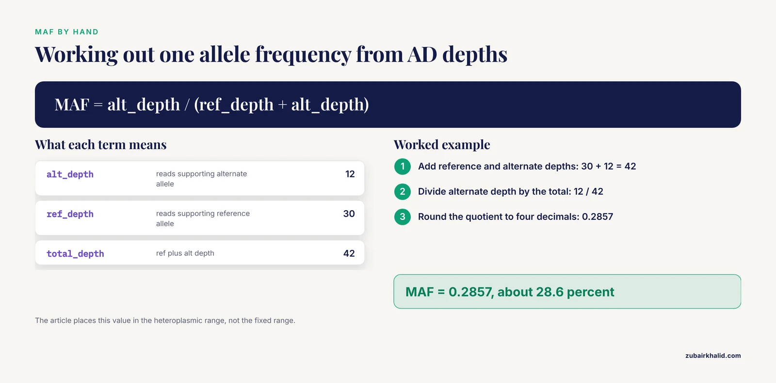
This step is the analytical core and mirrors the published Mito_Plot design. Mito_Plot calculates MAF based on allelic depth information from standard mitochondrial VCF files, then aggregates MAF values from multiple samples into a unified matrix aligned by genomic position, which enables direct cross-sample comparison across large cohorts [1].
MAF for a single sample and position is:
MAF = alt_depth / (ref_depth + alt_depth)The worked calculation for one record with a ref depth of 30 and an alt depth of 12 gives 12 / 42 = 0.2857, meaning roughly 28.6 percent of molecules at that position carry the alternate allele, which places the variant in the heteroplasmic range rather than the fixed range.
# src/03_maf_matrix.py
import argparse
from pathlib import Path
import pandas as pd

def compute_maf(df):
    df = df.copy()
    df["maf"] = df["alt_depth"] / df["total_depth"]
    return df

def build_matrix(frames: dict) -> pd.DataFrame:
    """frames maps sample_id -> filtered variant DataFrame."""
    tidy = []
    for sample_id, df in frames.items():
        m = compute_maf(df)
        tidy.append(m[["POS", "REF", "ALT", "sample", "maf"]])
    long = pd.concat(tidy, ignore_index=True)

    # Align every sample onto one shared genomic position axis.
    matrix = long.pivot_table(
        index=["POS", "REF", "ALT"],
        columns="sample",
        values="maf",
        aggfunc="mean",   # defensive: identical keys should not occur
    ).sort_index()

    # Deterministic column order.
    return matrix[sorted(matrix.columns)]

def main():
    ap = argparse.ArgumentParser()
    ap.add_argument("--indir", default="results/intermediate")
    ap.add_argument("--outdir", default="results/final")
    args = ap.parse_args()

    frames = {}
    for pq in sorted(Path(args.indir).glob("filtered_*.parquet")):
        sample_id = pq.stem.replace("filtered_variants_", "")
        frames[sample_id] = pd.read_parquet(pq)

    matrix = build_matrix(frames)
    outdir = Path(args.outdir)
    outdir.mkdir(parents=True, exist_ok=True)
    matrix.to_parquet(outdir / "maf_matrix.parquet")
    matrix.to_csv(outdir / "maf_matrix.csv", float_format="%.6f")
    print(matrix.round(3).head())
    print(f"matrix shape: {matrix.shape}")

if __name__ == "__main__":
    main()
Run it:
python src/03_maf_matrix.pyExpected output (numbers illustrative, shape depends on your data):
sample      sampleA  sampleB  sampleC
POS  REF ALT
3019 G    A      0.012    0.008      NaN
4769 A    G      0.286    0.291    0.302
10463 T   C      0.001      NaN    0.004
matrix shape: (147, 3)
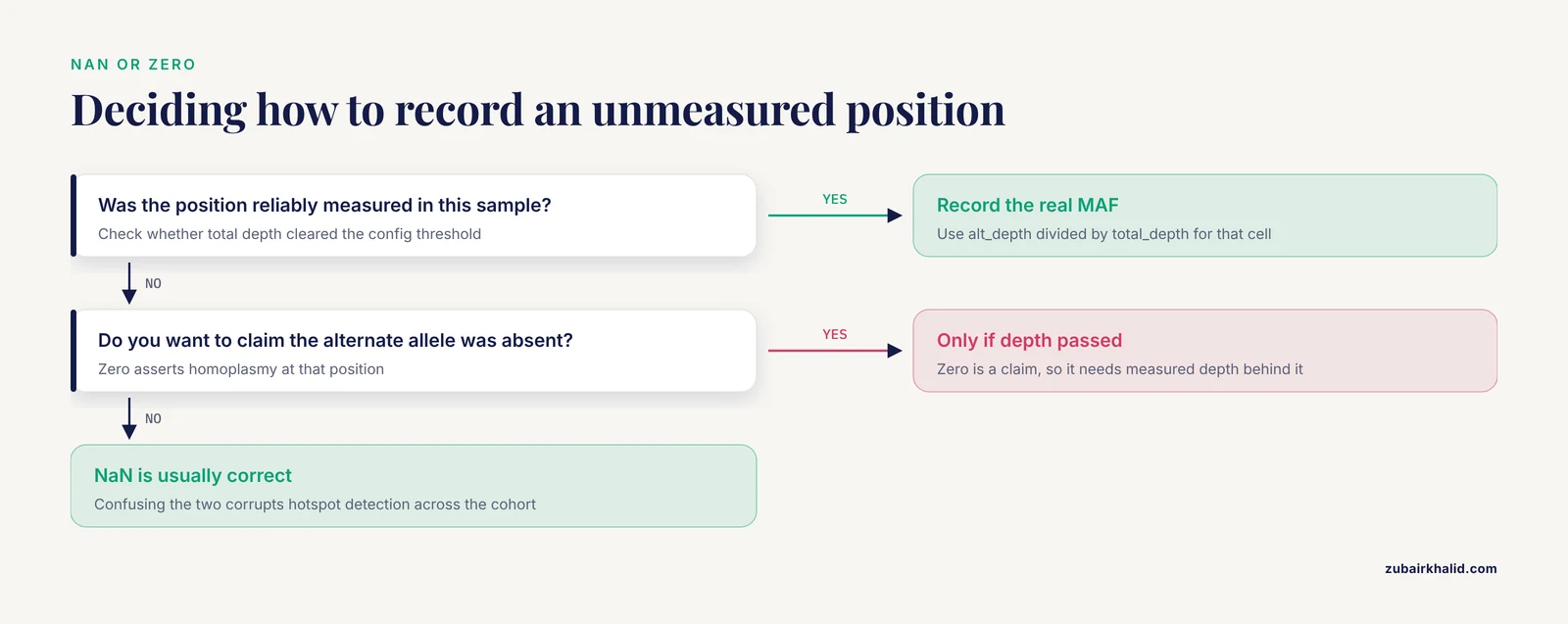
The NaN values are informative, not errors. They mark positions detected in some samples and not others, which usually means the position fell below the depth threshold in that sample. Deciding how to represent absence (NaN versus zero) is an analysis decision, not a pandas decision. Zero would falsely assert homoplasmy at an unobserved position, so NaN is usually correct.
Why a matrix and not a long table? The published Mito_Plot pipeline makes exactly this choice, aggregating MAF data from multiple samples into a unified matrix aligned by genomic position to enable direct cross-sample comparison and rapid identification of mutation hotspots and sample-specific patterns [1]. Wide matrices are also what plotting libraries, PCA, and clustering functions expect. Keep the long-format table alongside the matrix, because each format serves different downstream tools.
Step 7: Validate Before You Trust
Reproducibility includes proving the result is right, not just that it repeats. Add assertions that run on every execution:
# tests/test_maf.py
import numpy as np
import pandas as pd

def test_maf_bounds():
    df = pd.read_parquet("results/final/maf_matrix.parquet")
    vals = df.to_numpy().flatten()
    vals = vals[~np.isnan(vals)]
    assert (vals >= 0).all() and (vals <= 1).all(), "MAF outside [0, 1]"

def test_positions_sorted_unique():
    df = pd.read_parquet("results/final/maf_matrix.parquet").reset_index()
    assert df["POS"].is_monotonic_increasing
    assert not df.duplicated(subset=["POS", "REF", "ALT"]).any()

def test_sample_names_match_input():
    import glob, os
    inputs = {os.path.basename(p).replace("filtered_variants_", "").replace(".parquet", "")
              for p in glob.glob("results/intermediate/filtered_variants_*.parquet")}
    df = pd.read_parquet("results/final/maf_matrix.parquet")
    assert set(df.columns) == inputs, "samples lost or renamed during aggregation"

def test_maf_recalculation_spot_check():
    # Recompute MAF from depths for one known position and compare.
    per = pd.read_parquet("results/intermediate/filtered_variants_sampleA.parquet")
    row = per[per["POS"] == 4769].iloc
    expected = row["alt_depth"] / row["total_depth"]
    matrix = pd.read_parquet("results/final/maf_matrix.parquet")
    assert abs(matrix.loc[(4769, row["REF"], row["ALT"]), "sampleA"] - expected) < 1e-12
Run the tests after every change:
pytest tests/ -qA further cross-check that catches parser bugs early: extract the same fields with bcftools and compare row counts and a few spot values against your pandas output.
bcftools query -f '%POS\t%REF\t%ALT\t%AD\n' data/raw/sampleA.vcf | headIf bcftools reports 187 records and your parser reports 187 variants for sampleA, the counts agree. If they disagree, look first for multiallelic sites, where one VCF line carries two alternate alleles and naive AD parsing silently drops the second.
Step 8: Version, Checksum, and Orchestrate
Two final pieces make the pipeline a template others can adopt.
First, checksum the inputs and outputs:
md5sum data/raw/*.vcf > results/checksums_input.txt
md5sum results/final/* > results/checksums_final.txt
Commit both files. After a rerun, md5sum -c results/checksums_final.txt tells you in one command whether anything changed.
Second, wrap the numbered scripts in an orchestrator so the whole run is one command. A minimal Snakemake skeleton:
# Snakefile
SAMPLES = glob wildcards pattern here via glob_wildcards
rule all:
    input: "results/final/maf_matrix.parquet"

rule parse:
    input: "data/raw/{sample}.vcf"
    output: "results/intermediate/variants_{sample}.parquet"
    shell: "python src/01_parse_vcf.py --indir data/raw --outdir results/intermediate"

rule matrix:
    input: expand("results/intermediate/filtered_variants_{sample}.parquet", sample=SAMPLES)
    output: "results/final/maf_matrix.parquet"
    shell: "python src/03_maf_matrix.py"
The specific orchestrator matters less than the property it enforces: no step is run by hand, so no step can be forgotten, run out of order, or run against stale inputs.
Key pandas Options and Formulas for Genomic Pipelines
| Task | pandas tool | Parameter that matters | Why it matters for reproducibility |
|---|---|---|---|
| Read VCF or TSV | read_csv | sep="\t", comment="#", explicit dtype | Prevents inferred dtypes from drifting between files |
| Write outputs | to_parquet, to_csv | float_format="%.6f" on CSV | Fixes the number of printed digits so diffs are stable |
| Long to wide matrix | pivot_table | aggfunc, explicit index columns | Makes the aggregation rule explicit instead of implicit |
| Concatenating samples | concat | ignore_index=True, sorted inputs | Removes file-listing order dependence |
| Conditional assignment | .loc[mask, "col"] = v | None, never chained brackets | Avoids SettingWithCopyWarning and copy-on-write surprises |
| Joins with metadata | merge | validate="one_to_one" or "many_to_one" | Fails loudly if metadata has duplicate sample IDs |
| MAF formula | alt / (ref + alt) | Denominator from AD depths, not raw DP | Raw DP can include reads the AD field excludes |
| Group statistics | groupby | observed=True for categoricals | Prevents empty-category rows from appearing after upgrades |
Common Mistakes and Limitations
Mixing 1-based and 0-based coordinates. VCF is 1-based, BED and Python slicing are 0-based. Convert exactly once, at the parsing boundary, and add an assertion that POS values are at least 1 before conversion.
Parsing multiallelic sites naively. A VCF record like A -> G,T has AD with three values. Taking ad_idx value and splitting on commas gives three depths, and treating the second as "the alt depth" is wrong. Split the record with bcftools norm -m -any before pandas, or handle the extra depths explicitly.
Mutable input directories. A pipeline that writes filtered files into data/raw will, on the second run, parse its own outputs. Keep raw data read-only and write everything under results/.
Nondeterministic file ordering. glob() and os.listdir() return arbitrary order on some filesystems. Always sorted(). Then aggregate columns or rows in a fixed order.
Chained assignment. df[mask]["maf"] = x is the single most common pandas bug in analysis scripts. It can appear to work, warn, or silently do nothing depending on the pandas version. Use .loc or .copy().
Silent index alignment in arithmetic. df1["maf"] - df2["maf"] aligns on the index, not on row order. If two frames have differently ordered or partially overlapping positions, you get NaNs where the analyst expected numbers. Reindex explicitly before arithmetic.
NaN versus zero for absent observations. Zero asserts the position was measured and the alternate allele was absent. NaN asserts the position was not reliably measured. In allele frequency work these are different biological claims, and confusing them corrupts hotspot detection.
Overloading one notebook. A 400-cell notebook that parses, filters, aggregates, and plots is not a pipeline, because its state depends on the order in which cells were run. Split it into the numbered scripts above and let the notebook only call them.
Limitations of the approach itself. pandas holds data in memory, so whole-genome matrices with millions of positions and thousands of samples will not fit on a laptop. For those scales, chunk by genomic region or move to tools designed for out-of-core data, keeping pandas for the per-chunk tidy operations it excels at. Also, this pattern assumes clean, complete metadata. If sample IDs are inconsistent between the VCF filenames and the phenotype sheet, add a validation step that fails before any analysis, not after.
Frequently Asked Questions
What does a reproducible genomic analysis pipeline with pandas actually require?
Four things: a pinned software environment, deterministic code with fixed seeds and sorted file handling, a declared input format contract, and a single command that runs every step in order. Provenance files recording versions and checksums make the rerun verifiable rather than merely claimed.
Is there a complete reproducible genomic analysis pipeline pandas example I can copy?
Yes, the eight-step walkthrough in this article is a complete example, from parsing VCF files through building a position-aligned MAF matrix to validation tests and checksums. Each script is self-contained and the directory layout doubles as the template.
What file format should a reproducible genomic analysis pipeline pandas project use for inputs and outputs?
Use standard community formats at the boundaries, such as VCF for variants and FASTA for reference sequences, and convert once into tidy DataFrames internally. For intermediate and final outputs, prefer parquet for type fidelity plus a CSV copy with a fixed float format for human review.
Can I get a reproducible genomic analysis pipeline pandas template for my own project?
Yes, the directory layout in Step 2, the numbered scripts in Steps 4 through 6, the config file, and the test file together form a working template. Rename the project folder, swap in your own data files, and adjust the thresholds in config.yaml.
How much Python do I need for python for bioinformatics work?
You need intermediate core Python plus a working command of pandas indexing, boolean masks, groupby, and merge, and comfort reading tool documentation. You do not need software engineering expertise, but you do need the discipline to write functions and scripts instead of one long interactive session.
Do I need Biopython if I am mainly using pandas?
Use Biopython whenever your workflow reads or writes biological file formats such as FASTA, GenBank, or BLAST outputs. For a project that only consumes already-extracted VCF tables, you can skip it, but most genomic projects touch at least one sequence file, so it is usually installed anyway.
How does the MAF calculation work in a mitochondrial heteroplasmy pipeline?
MAF is the alternate allele depth divided by the sum of reference and alternate depths at that position. The Mito_Plot pipeline computes it from the allelic depth information in standard mitochondrial VCF files and then aligns the values across samples by genomic position for cohort-level comparison.
How do I verify my pandas pipeline gives the same results on another machine?
Pin the environment, record input and output checksums, run pytest after the rerun, and spot-check a few values against an independent tool such as bcftools. If the checksums match and the tests pass, the rerun reproduced the original analysis.