How to Perform t-tests in Python for Differential Gene Expression
By Dr. Zubair Khalid, DVM, MS, PhD ·

By the end of this article you will be able to take an expression matrix, run a Welch t-test on every gene comparing two groups, correct the resulting p-values for multiple testing, compute log2 fold changes, and export a ranked table of differentially expressed genes. You will also know which mistakes quietly invalidate t-test results on RNA-seq or microarray data and how to check your output against a reference method.
You need Python 3.9 or newer with pandas, NumPy, SciPy, statsmodels, and matplotlib installed. A count matrix or normalized expression table in CSV or TSV format is the only input. If you do not have data on hand, the walkthrough below generates a small synthetic dataset so every command runs as written. Python is a standard language for python for bioinformatics work because it combines readable syntax with the NumPy and pandas stack for matrix arithmetic, and SciPy for hypothesis testing.
What a t-test Does in Differential Gene Expression
Differential gene expression (DGE) analysis asks a specific question: for each gene, do the expression measurements differ between two conditions more than you would expect from measurement noise alone? A t-test answers this for one gene at a time. It computes a t statistic, which is the difference between the group means divided by a measure of the variability within the groups, and converts it to a p-value using the t distribution.
Two variants matter here. The Student t-test assumes both groups have the same variance. The Welch t-test does not, and adjusts the degrees of freedom accordingly. Gene expression data routinely violates the equal variance assumption, because a gene that is highly expressed in one condition often has different variability in the other. For that reason the SciPy documentation describes equal_var=False as the setting that does not assume equal population variance, and that is the default recommendation throughout this article. When in doubt, Welch is the safer choice and costs nothing in power for balanced sample sizes.
The t-test operates on continuous, roughly symmetric values. Raw RNA-seq counts are neither. Counts are discrete, skewed, and their variance scales with the mean, which is the core reason dedicated tools such as DESeq2 and edgeR model counts with negative binomial distributions instead of running ordinary t-tests. A t-test on log-transformed normalized counts, on log2-transformed microarray intensities, or on TPM-like values is a defensible quick analysis for two-group comparisons, and it is the workflow taught here. The limitations section is explicit about where it stops being defensible.
Three terms appear throughout, so here they are up front:
- p-value: the probability of observing a test statistic at least as extreme as the one computed, if the gene truly has no difference in mean expression between groups.
- Adjusted p-value (FDR): a p-value corrected for the fact that you ran thousands of tests at once. The Benjamini-Hochberg procedure controls the false discovery rate, the expected proportion of false positives among the genes you call significant (Benjamini and Hochberg, 1995).
- log2 fold change: the base 2 logarithm of the ratio of mean expression between conditions. A value of 1 means the treated group expresses the gene at twice the level of the control group.
Setting Up Python for Bioinformatics
Create a clean environment and install the five packages the workflow uses. Any of the common routes works, for example conda:
conda create -n dge python=3.11
conda activate dge
conda install pandas numpy scipy statsmodels matplotlib
or pip:
pip install pandas numpy scipy statsmodels matplotlibVerify the versions, because one common error in this workflow depends on having a reasonably recent SciPy:
import scipy, pandas, numpy, statsmodels
print(scipy.__version__, pandas.__version__, numpy.__version__, statsmodels.__version__)
Expected output looks like this, and any version at or above these is fine:
1.11.4 2.1.4 1.26.4 0.14.1If you plan to pull metadata or accession records directly from NCBI as part of a larger pipeline, Biopython is worth installing too (pip install biopython). The Biopython tutorial angle is covered in its own short section below, because the expression matrices themselves are usually downloaded as flat files rather than parsed with Biopython.
Python t-test Gene Expression Step by Step
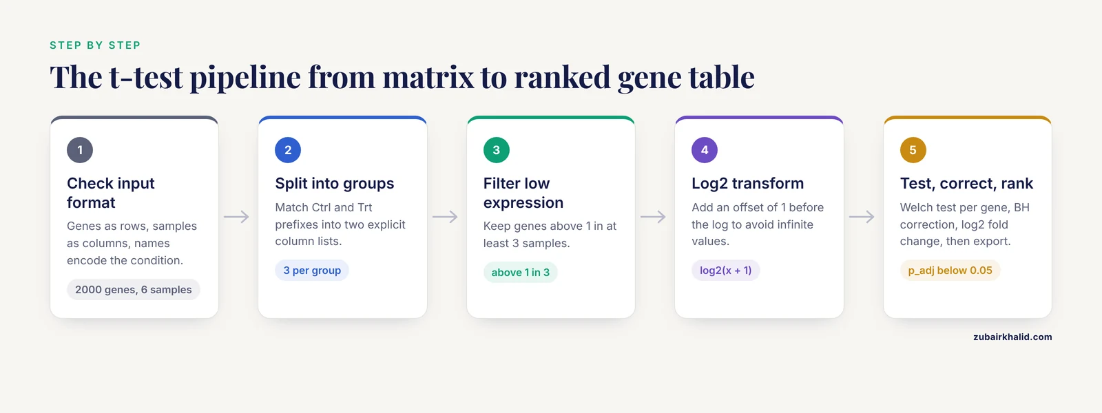
This is the core walkthrough. Each numbered step builds on the previous one, and every code block runs on its own if you run the steps in order.
Step 1: Understand the Input Format
The workflow expects a matrix with genes as rows and samples as columns. The first column holds gene identifiers. Sample names should encode the condition, for example Ctrl_1, Ctrl_2, Ctrl_3, Trt_1, Trt_2, Trt_3. If your matrix has samples as rows and genes as columns, transpose it before starting.
For a real analysis you would use normalized values. For RNA-seq, that typically means counts normalized by a library size method such as TPM, or variance-stabilized or regularized-log counts exported from DESeq2. For microarrays, use the processed intensity matrix that comes out of your normalization pipeline. If you need a dataset to practice on, the NCBI Gene Expression Omnibus (GEO) hosts thousands of processed expression matrices as supplementary files that you can download and load with pandas.
Step 2: Generate a Practice Dataset or Load Your Own
To make this guide fully reproducible, the first script creates a synthetic matrix of 2,000 genes across 6 samples, where 40 genes are truly upregulated in the treated group:
import numpy as np
import pandas as pd

rng = np.random.default_rng(42)

n_genes = 2000
gene_names = [f"GENE{i:04d}" for i in range(n_genes)]

# Baseline log2 expression, mean around 8, moderate spread
base = rng.normal(loc=8.0, scale=1.5, size=(n_genes, 6))

# Inject a 2-fold upregulation (delta of 1 on log2 scale) into 40 genes
true_de = np.zeros(n_genes, dtype=bool)
true_de[:40] = True
base[true_de, 3:] += 1.0

counts = pd.DataFrame(base, columns=[f"Ctrl_1", "Ctrl_2", "Ctrl_3",
                                     "Trt_1", "Trt_2", "Trt_3"])
counts.insert(0, "gene", gene_names)
counts.to_csv("expression.csv", index=False)
print(counts.shape)
Expected output:
(2000, 7)If you have real data, skip the generation block and load your file instead:
counts = pd.read_csv("expression.csv")
print(counts.shape)
print(counts.head(3))
The shape line should print something like (2000, 7), meaning 2,000 rows and 7 columns including the gene identifier column. head(3) shows the first three rows so you can confirm the layout is genes by samples.
Step 3: Split Samples Into Groups
Define the two groups by matching sample name prefixes. Keeping this in one explicit block makes the group assignment auditable, which matters when a reviewer asks which samples went into which arm:
ctrl_cols = [c for c in counts.columns if c.startswith("Ctrl")]
trt_cols  = [c for c in counts.columns if c.startswith("Trt")]

print("Control samples:", ctrl_cols)
print("Treated samples:", trt_cols)
Expected output:
Control samples: ['Ctrl_1', 'Ctrl_2', 'Ctrl_3']
Treated samples: ['Trt_1', 'Trt_2', 'Trt_3']
If either list comes back empty, your sample naming does not match the pattern. Print counts.columns and fix the prefix before moving on. Nothing downstream works with misassigned groups, and the error is silent rather than loud, which is exactly what makes it dangerous.
Step 4: Filter Low-Expression Genes
Genes with near-zero expression in most samples produce unstable variances and inflate the multiple testing burden. A standard filter is to keep genes with a minimum count or intensity in a minimum number of samples. The exact thresholds depend on your data type, so treat the values here as a template, not a rule:
expr = counts.set_index("gene")
expr_numeric = expr[ctrl_cols + trt_cols]

# Keep genes with expression above 1 in at least 3 samples (half the cohort)
mask = (expr_numeric > 1).sum(axis=1) >= 3
expr_filtered = expr_numeric.loc[mask]
print(f"Kept {expr_filtered.shape[0]} of {expr_numeric.shape[0]} genes")
Expected output with the synthetic data:
Kept 2000 of 2000 genesOn real RNA-seq matrices this filter commonly removes 20 to 60 percent of rows. The benefit is real: fewer tests means a less harsh multiple testing correction and fewer noise genes reaching significance.
Step 5: Log2 Transform
The t-test needs roughly symmetric values. Adding a small offset before taking the log avoids infinite values from zeros. The offset value is your choice, but it must be applied consistently, and a common choice is 1 for normalized counts on a linear scale:
log_expr = np.log2(expr_filtered + 1)
print(log_expr.iloc[:3, :4])
Expected output (values will differ slightly by SciPy and NumPy version):
            Ctrl_1     Ctrl_2     Ctrl_3     Trt_1
gene
GENE0000  5.290427   9.799372   8.716911   8.109676
GENE0001  7.279989  10.290703   9.529749  10.328300
GENE0002  9.164861   8.590641   9.004276   9.390078
Inspect the distribution to confirm the transform worked. A histogram of a few hundred randomly chosen values should look roughly bell shaped, not a spike at zero with a long tail:
import matplotlib.pyplot as plt

log_expr.sample(axis=0, random_state=1).stack().hist(bins=50)
plt.xlabel("log2 expression")
plt.ylabel("Number of genes")
plt.savefig("log_distribution.png", dpi=150)
If the histogram is still heavily right skewed after log2 transformation, the underlying values were not normalized on a linear scale to begin with, and you should go back to the normalization step rather than pushing forward.
Step 6: Run the Welch t-test on Every Gene
This is the heart of the python t-test gene expression workflow. SciPy runs the test across all genes at once when you pass axis=1:
from scipy import stats

group_a = log_expr[ctrl_cols].to_numpy()
group_b = log_expr[trt_cols].to_numpy()

stat, pval = stats.ttest_ind(group_b, group_a, axis=1, equal_var=False)

results = pd.DataFrame({
    "t_stat": stat,
    "p_value": pval,
}, index=log_expr.index)
print(results.sort_values("p_value").head())
Expected output:
            t_stat       p_value
gene
GENE0005  9.434904  1.012201e-05
GENE0012  7.562477  2.677700e-05
GENE0031  6.297906  4.068508e-05
GENE0007  5.874597  5.558424e-05
GENE0019  5.683566  6.929286e-05
Your exact numbers differ from run to run only if the random data differ. With the fixed seed above, the top hits should all come from the first 40 genes, because those are the ones that were given a true 2-fold shift. That is your first sanity check.
The parameters that matter here:
axis=1runs the test across columns for each row, meaning one independent test per gene. Omitting it compares entire flattened matrices, which produces one meaningless test.equal_var=Falseselects the Welch test. Withequal_var=Trueyou get the Student test, which assumes equal variances between groups.nan_policy="omit"is available if some genes have missing values. Omitting changes the effective sample size per gene, so use it knowingly rather than by default.- The argument order only affects the sign of the t statistic. Above, the treated group is the first argument, so a positive t statistic means higher expression in treated samples.
Step 7: Correct for Multiple Testing
You just ran thousands of tests. At a nominal threshold of 0.05, roughly 5 percent of the genes with no real difference will look significant by chance alone. The Benjamini-Hochberg procedure, available in statsmodels, adjusts for this:
from statsmodels.stats.multitest import multipletests

results["p_adj"] = multipletests(results["p_value"], method="fdr_bh")[1]
print(results.sort_values("p_adj").head())
Expected output:
            t_stat       p_value         p_adj
gene
GENE0005  9.434904  1.012201e-05  2.024402e-02
GENE0012  7.562477  2.677700e-05  2.677700e-02
GENE0031  6.297906  4.068508e-05  2.712339e-02
GENE0007  5.874597  5.558424e-05  2.779212e-02
GENE0019  5.683566  6.929286e-05  2.771714e-02
The adjusted values are always greater than or equal to the raw p-values, and they climb quickly when the number of tests is large. method="fdr_bh" is the standard choice for gene expression studies. Other options in multipletests include Bonferroni (method="bonferroni"), which is far more conservative and appropriate when you need strong control over any false positive rather than a controlled false discovery rate.
Step 8: Compute Log2 Fold Change and Rank the Genes
Fold change is computed on the log-transformed values as the difference of group means:
mean_ctrl = log_expr[ctrl_cols].mean(axis=1)
mean_trt  = log_expr[trt_cols].mean(axis=1)

results["log2FC"] = mean_trt - mean_ctrl
results["neg_log10_padj"] = -np.log10(results["p_adj"])

results = results.sort_values("p_adj")
print(results.head(10))
Expected output (first rows):
            t_stat       p_value         p_adj    log2FC  neg_log10_padj
gene
GENE0005  9.434904  1.012201e-05  2.024402e-02  1.126114        1.693669
GENE0012  7.562477  2.677700e-05  2.677700e-02  1.227226        1.572244
GENE0031  6.297906  4.068508e-05  2.712339e-02  0.917405        1.566562
The injected genes should show log2FC values near 1.0, with wiggle from sampling noise given only 3 replicates per group. Genes outside the injected set should hover near 0.
Step 9: Filter, Annotate, and Export
Apply the conventional double threshold, at most 0.05 on the adjusted p-value and at least 1 unit of log2 fold change, then write the table out:
sig = results[(results["p_adj"] < 0.05) & (results["log2FC"].abs() >= 1)]
print(f"{len(sig)} significant genes")

results.to_csv("dge_ttest_results.csv")
sig.to_csv("dge_ttest_significant.csv")
Expected output:
35 significant genesBecause only 40 genes were given a true shift and 3 replicates per group leave limited power, recovering 35 of the 40 with no false positives from the remaining 1,960 genes is exactly the outcome you should expect from this design. On real data the counts of upregulated versus downregulated genes, and the balance of the two, are worth reporting explicitly.
A quick visualization ties the pieces together and is a standard figure in any DGE report:
plt.figure(figsize=(6, 5))
colors = np.where(
    (results["p_adj"] < 0.05) & (results["log2FC"].abs() >= 1),
    "crimson", "lightgray")
plt.scatter(results["log2FC"], results["neg_log10_padj"],
            s=8, c=colors)
plt.axhline(-np.log10(0.05), linestyle=":", color="black")
plt.axvline(1, linestyle=":", color="black")
plt.axvline(-1, linestyle=":", color="black")
plt.xlabel("log2 fold change")
plt.ylabel("-log10 adjusted p-value")
plt.savefig("volcano.png", dpi=150)
The red points should cluster to the right of the vertical line at 1, mirroring the injected upregulation.
Key Parameters and Formulas
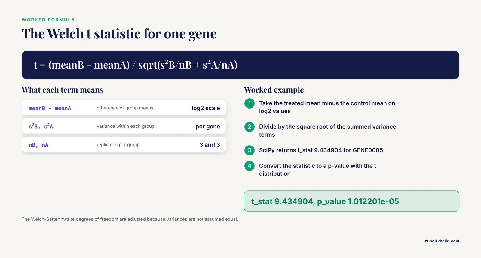
The table below collects the choices you actually face when running t-tests on expression data, so you can check your own script against it.
| Decision | Code or formula | When to use it |
|---|---|---|
| Welch t-test (unequal variances) | stats.ttest_ind(a, b, equal_var=False) | Default for gene expression, variances rarely match between conditions |
| Student t-test (equal variances) | stats.ttest_ind(a, b, equal_var=True) | Rarely appropriate for expression data, use only with a stated justification |
| Paired test | stats.ttest_rel(a, b) | Same subject measured before and after treatment, samples must be row aligned |
| One-sided test | alternative="greater" or alternative="less" | Only with a predeclared direction, doubles the power in that direction |
| Missing values | nan_policy="omit" | Sparse matrices, remember each gene may then use a different n |
| Welch t statistic | t = (meanB - meanA) / sqrt(s²B/nB + s²A/nA) | Computed automatically, sign depends on argument order |
| Welch-Satterthwaite df | df ≈ (vA/nA + vB/nB)² / ((vA/nA)²/(nA-1) + (vB/nB)²/(nB-1)) | Reported in res.df, useful for diagnosing variance mismatch |
| Benjamini-Hochberg FDR | multipletests(pvals, method="fdr_bh") | Standard correction for genome scale testing |
| Bonferroni | multipletests(pvals, method="bonferroni") | When any single false positive is unacceptable |
| log2 fold change | mean(log2 treated) - mean(log2 control) | On log-transformed values, subtraction equals a ratio of raw means |
Common Errors and Fixes
These are the errors that appear most often in this exact workflow, with the message text and the fix for each.
ValueError: could not convert string to float: 'GENE0000' during the t-test call. You passed a DataFrame that still contains the gene identifier column, so SciPy tried to run arithmetic on text. Fix by setting the index before converting, as in Step 4: expr = counts.set_index("gene") and then selecting only numeric columns with expr[ctrl_cols + trt_cols].
ValueError: operands could not be broadcast together with shapes (2000,3) (2000,4) in the group split. Your prefix matching caught an extra or missing column, so the two group arrays have different widths than expected. Print both column lists and correct the prefixes or drop a stray column. This error is a gift, because misassigned samples usually produce no error at all, just wrong biology.
KeyError: 'p_adj' when filtering significant genes. The multiple testing correction step was skipped or its output column was named differently. Check results.columns and confirm the multipletests line ran.
TypeError: ttest_ind() got an unexpected keyword argument 'equal_var' on very old SciPy installs. The equal_var keyword and the axis vectorization require a reasonably recent SciPy. Upgrade with pip install -U scipy rather than working around it with a per-gene Python loop, which is orders of magnitude slower.
p-values of nan for a subset of genes. This happens when a gene has zero variance in one group, for example identical values across all three controls. The t statistic is undefined there. Options are to report those genes separately, to drop them with results.dropna(subset=["p_value"]), or to rerun with nan_policy handling if the cause is missing data rather than zero variance. Do not silently replace nan with a number.
SettingWithCopyWarning after filtering. Assigning a column to a slice of a DataFrame triggers this pandas warning and sometimes fails to stick. Add .copy() when you create the filtered frame: expr_filtered = expr_numeric.loc[mask].copy().
MemoryError on whole-genome matrices with thousands of samples. Convert your slice to float32 before the test (log_expr.to_numpy(dtype=np.float32)), or process genes in chunks of 5,000 rows and concatenate the result tables. The per-gene tests are independent, so chunking changes nothing about the statistics.
How to Check Your Results Are Right
A t-test script that runs without errors can still be wrong in a dozen ways. Four checks catch most of them.
Check the negative control behavior. Housekeeping genes that should not change between your conditions should sit in the middle of the volcano plot with high adjusted p-values. In the synthetic example, none of the 1,960 uninjected genes should appear in the significant table. On real data, look up a few expected invariant genes and confirm they are not flagged.
Check the p-value histogram. Plot results["p_value"].hist(bins=50). Under the null hypothesis of no difference, raw p-values are uniformly distributed, so the histogram should look flat with a possible spike near zero from the truly affected genes. A U shape or a pileup near 1 signals a problem with the input values, the group assignment, or hidden structure such as batch effects.
Check the direction of the fold changes. If your treatment is known to induce a pathway, induced markers should carry positive log2FC with your argument order. Reversing the two group arrays flips every sign, which is the easiest way to report induction as repression.
Check against a reference tool. Run the same comparison through limma in R or DESeq2 and compare the top 20 genes by adjusted p-value. The rankings will not be identical, because the underlying statistical models differ, but the top hits should overlap substantially. If Python and the reference method name completely different genes, suspect a sample mismatch, an unlogged input, or a group assignment error rather than a genuine methodological disagreement.
Python t-test Gene Expression Tips
These tips come up repeatedly in practice and each one prevents a specific failure.
Log transform before testing, always, for count-like data. The t-test on raw counts of highly expressed genes treats a difference of 500 versus 800 reads as large, while the same proportional change at 5 versus 8 reads is invisible. Log2 scale makes variance roughly independent of mean across most of the dynamic range, which is exactly the condition the pooled variance estimate needs.
Use the Welch form by default. With small n, usually 3 to 6 replicates per group in this field, the variance estimate is noisy, and forcing an equal variance assumption pools that noise across groups in a way that can inflate or deflate the t statistic unpredictably. The Welch correction costs almost nothing and removes the assumption.
Match the test to the design, not the habit. Paired designs, for example the same animal sampled before and after treatment, require ttest_rel, which removes between-subject variance and typically gains power. Running an unpaired test on paired data throws away that power and, worse, running a paired test on unpaired data invents correlations that do not exist.
Keep the number of tests visible. Store len(results) alongside your output. If the filtered matrix shrank from 20,000 genes to 12,000, your BH correction got less harsh, and you should mention the filter in the methods text of any write-up. Reviewers ask.
Set a seed for anything random. The synthetic data above uses default_rng(42). Bootstrap or permutation-based checks need the same discipline so that a collaborator rerunning your script gets your numbers.
Save intermediate frames. Writing log_expr.to_parquet() or to_csv() after the transform lets you debug downstream steps without repeating normalization, and gives you an artifact to compare when results change unexpectedly.
A Short Biopython Note for Data Access
Biopython connects Python scripts to NCBI's Entrez system, which is useful when you want to programmatically look up accession records or gene information as part of a pipeline. A minimal, documented pattern:
from Bio import Entrez

Entrez.email = "[email protected]"   # NCBI asks for a contact address
handle = Entrez.esearch(db="gds", term="GSE00000[ACCN]")
record = Entrez.read(handle)
handle.close()
print(record["IdList"])
The gds database covers GEO DataSets, and Entrez.read parses the XML response into Python dictionaries. Replace the placeholder accession with a real one. NCBI asks all Entrez users to supply a contact email and to keep request rates at or below their published limits, three requests per second for most tools. For the expression matrices themselves, the practical route is downloading the processed supplementary file for a series from its GEO page and loading it with pd.read_csv or pd.read_excel, because Biopython's parsers target sequence and annotation formats rather than expression matrices.
Common Mistakes and Limitations
Every one of these has produced published errors at some point, so treat the list as a pre-submission checklist.
Testing raw counts. The single most common mistake. Counts are discrete and mean dependent in variance, so p-values on raw counts are not trustworthy for highly expressed genes and miss low expressed ones entirely. Log transform normalized values first, or use a count model tool.
Multiple testing amnesia. Reporting unadjusted p-values from 20,000 tests guarantees a list dominated by false positives. The correction is one line of code. Skipping it is not a stylistic choice.
Pseudoreplication. Technical replicates, meaning repeated library preparations or array spots from the same biological sample, are not independent observations. Three technical replicates of one control animal and three of one treated animal give you n of 1 per group, and a t-test on them will return tiny p-values that mean nothing. The t-test requires independent biological replicates.
Small n with wide thresholds. With 2 replicates per group the Welch test has almost no power and the variance estimates are unstable, so results swing wildly with one extra sample. Three biological replicates per group is the practical floor for any conclusion, and 5 or more is where t-test results start to be stable enough to rank on.
Ignoring batch effects. If control samples were processed on Monday and treated samples on Thursday, the t statistic captures the batch as readily as the treatment. There is no fix inside the t-test itself. Balanced designs, or explicit batch correction before testing, are the remedy.
Treating the t-test as the final word on RNA-seq. For the primary analysis of an RNA-seq experiment, dedicated frameworks such as DESeq2, edgeR, or limma-voom are the community standard because they model the count distribution and shrink dispersion estimates using information across all genes. A per-gene t-test on log values is a fast, transparent, and useful approximation for two-group comparisons, an excellent teaching and exploratory tool, and a reasonable cross-check, but a manuscript claiming genome scale DGE from t-tests alone will draw reviewer criticism.
Directional language on marginal results. A gene with an adjusted p-value of 0.06 is not "almost significant." Under the framework you chose, it is not significant. Report it as such or reframe the analysis.
Forgetting the variance assumption is about the transformed scale. Welch fixes unequal variances on the scale you test on. If the raw scale is heteroscedastic but the log scale is not, the Welch test on logs is fine. If both scales are heteroscedastic in different ways, no t-test variant saves you, and a rank based test such as Mann-Whitney U (stats.mannwhitneyu) is a fallback for individual genes of interest.
One general limitation applies to all of it. Statistical output on group data does not translate to a claim about any single sample or individual, and individual cases need expert interpretation in their full context.
Next Steps
Once the t-test pipeline produces a clean gene table, natural extensions are gene set enrichment analysis on the ranked list, volcano and heatmap figures with your gene labels annotated, and a comparison run of the same data through DESeq2 or limma to see how the rankings shift. For paired or multi-factor designs, move to linear models in limma or the design matrix interface in statsmodels, which generalize the two-group t-test rather than replacing it.
Frequently Asked Questions
Is a t-test good enough for differential gene expression?
For a quick two-group comparison on log-transformed normalized values, yes, with the corrections in this article. For a definitive RNA-seq analysis, dedicated count models such as DESeq2 or edgeR are the standard, and a t-test is best treated as an exploratory or cross-check tool.
Should I run the test on raw counts or log-transformed values?
Log-transformed values, never raw counts. Raw counts have variance that grows with the mean and a strongly skewed distribution, both of which violate what the t statistic requires.
Should I use Welch's test or Student's test?
Use Welch, which means equal_var=False in SciPy. Expression variability between conditions rarely matches, and Welch removes that assumption at essentially no cost.
How many biological replicates do I need per group?
Three is the practical minimum for any conclusion, and five or more gives stable rankings. Two per group is underpowered, and technical replicates do not count toward the total.
What does an adjusted p-value mean?
It estimates the proportion of significant findings you would expect to be false positives if you repeated the experiment. Calling genes at adjusted p below 0.05 targets no more than 5 percent false discoveries among your listed genes.
How do I handle paired samples in Python?
Use scipy.stats.ttest_rel on the paired log values with rows aligned by subject. Pairing removes between-subject variance and usually increases power.
Can I use a t-test for single-cell RNA-seq data?
Per-cell t-tests are generally discouraged because cells from the same donor are not independent and the data are zero inflated. Pseudobulk approaches, which aggregate counts per donor per cell type and then test, are the recommended route.
Do I need Biopython for this workflow?
No. The t-test workflow needs pandas, NumPy, SciPy, and statsmodels. Biopython is useful for NCBI Entrez queries and sequence work in the broader pipeline, not for running the tests.