How to Plot Genomic Data Along Chromosomes in R with karyoploteR
By Dr. Zubair Khalid, DVM, MS, PhD ·

By the end of this karyoploteR tutorial you will be able to take a table of variants, peaks, or copy-number segments and turn it into a finished chromosome-scale figure: a base karyotype with ideograms, overlaid points and density curves, gene markers, base-pair axis ticks, a zoomed locus panel, and a high-resolution export for a manuscript or report.
Here is what you need on hand before starting:
- A recent R installation. Bioconductor releases are tied to R versions, so use a current release rather than an old one.
- The karyoploteR package from Bioconductor, plus regioneR and GenomicRanges, which arrive automatically as dependencies.
- Optional but recommended for real data: vcfR for VCF files, rtracklayer for bigWig files, and Rsamtools for BAM coverage.
- About 20 minutes for the first walkthrough and a few hundred megabytes of disk space for the dependency stack.
karyoploteR is an R package distributed through Bioconductor, the open-source software project that anchors much of the standard R for bioinformatics ecosystem. The problem it solves is specific. ggplot2 excels at abstract axes, but genomic figures usually need one axis to be the chromosome itself, with bands, centromeres, and true physical scale. karyoploteR draws that chromosome scaffold for you and lets you paint any interval data onto it. Chromosome maps like this have become a standard way to communicate genomics, from interactive tools such as the yEvo Mutation Browser, which places mutations from experimentally evolved yeast populations on a chromosome map so students can see where each mutation landed [1], to published cancer genomics studies that assemble their figures from R packages such as ggplot2, dplyr, ggrepel, and tidyr [2]. karyoploteR covers the part of that space that ggplot2 does not handle well: data placed on chromosomes, to scale.
What karyoploteR Does and When to Reach for It
A karyotype is a standardized cartoon of an organism's chromosomes, and an ideogram is the drawing of one chromosome, usually decorated with cytobands, the light and dark staining bands cytogeneticists use as landmarks such as 17p13 or 8q24. karyoploteR builds these ideograms for you and then overlays your data. Every position is a real genomic coordinate, so a point at chr1:150,000,000 lands at the correct physical position along the chr1 ideogram.
Choose karyoploteR when you need any of the following:
- A genome-wide overview of where your features sit: mutations, GWAS hits, ChIP peaks, copy-number segments, QTL.
- A multi-track figure comparing several data types or several samples on the same chromosomes.
- A scripted, reproducible figure. Because the plot is code, regenerating it after a pipeline rerun costs nothing.
- Figures for small or non-model genomes that genome browsers handle awkwardly.
Reach for something else when you need interactivity or base-resolution browsing. Desktop and web genome browsers are better for exploratory scrolling, and Shiny applications built for variant review, such as XVCF, which wraps vcfR and maftools behind a graphical interface for VCF summarization and quality control [3], are better for point-and-click exploration. karyoploteR is the scripted, static, publication-oriented member of that family. The broader trend in R favors exactly this kind of integration, where analysis and publication-ready regional visualization live in one toolkit, as LDblockR does for linkage disequilibrium analysis [4]. karyoploteR fills that same integration role for chromosome-scale plots.
Installing karyoploteR with Bioconductor
The install is the slowest step in this Bioconductor tutorial because karyoploteR pulls in a stack of genomics dependencies.
install.packages("BiocManager")
BiocManager::install("karyoploteR")
Install the companions used in this guide:
BiocManager::install(c("regioneR", "GenomicRanges", "GenomeInfoDb"))
BiocManager::install(c("Rsamtools", "rtracklayer", "VariantAnnotation"))
install.packages("vcfR")
regioneR and GenomicRanges install automatically with karyoploteR, but listing them makes each script's intent explicit. On Windows and macOS, binary packages install without compilation. On Linux, packages such as Rsamtools and rtracklayer compile from source and need standard build tools and development headers, so expect the first install to take several minutes.
Confirm everything loads:
library(karyoploteR)
library(regioneR)
packageVersion("karyoploteR")
The console prints the installed version number. Versions advance with each Bioconductor release, so any recent version is fine.
One habit separates reproducible figure scripts from one-off sessions. Record the environment at the bottom of every analysis script with sessionInfo(), and keep the entire figure, from file import to dev.off(), inside one script. Fragmented tooling spread across languages and ad hoc conversion steps is a documented source of reproducibility and provenance trouble in population genomics workflows [5], and a plotting script is the easiest place to avoid that failure mode.
Core Concepts: The KaryoPlot Object, Data Panels, and the r0 and r1 System
Three ideas explain almost everything about how karyoploteR works.
The KaryoPlot object. plotKaryotype() draws the chromosome scaffold and returns an object, conventionally assigned to a variable named kp. Every later function takes kp as its first argument and draws onto the existing figure immediately, in the style of base R graphics rather than ggplot2. Nothing is buffered, so the order of your calls is the order of your layers, and every call must happen while the graphics device is open.
Data panels. Most layouts provide one or two horizontal strips beside the ideograms where data lives. Data panel 1 sits above the ideograms and data panel 2 below them, depending on plot.type. Every data function accepts a data.panel argument, so the same GRanges object can be drawn twice, once in each panel, with different representations. By default, drawing is clipped to the plotted window, so features outside the visible chromosomes simply do not appear.
The r0 and r1 coordinate system. Within a data panel, vertical position is expressed as a fraction from 0 at the bottom to 1 at the top. r0 sets the bottom of a track and r1 sets the top. A track with r0=0 and r1=0.5 fills the lower half of the panel. Stack tracks by giving each a disjoint r0 to r1 slice. For value-drawing functions such as kpPoints and kpLines, the y argument is also expected between 0 and 1, and karyoploteR scales it into the r0 to r1 window. Normalize real measurements before passing them.
Table 1 summarizes the functions you will use most.
| Function | What it draws | Key arguments |
|---|---|---|
| plotKaryotype() | Base karyotype and ideograms | genome, custom.genome, plot.type, zoom, plot.params, chromosomes |
| kpDataBackground() | Shaded background for a track | data.panel, r0, r1, color |
| kpPoints() | Points at genomic positions | data, y, r0, r1, col, pch, cex |
| kpLines() | Line through genomic values | data, y, r0, r1, col, lwd |
| kpRect() | Filled rectangle spanning each interval | data, r0, r1, col, border |
| kpSegments() | Vertical bar for each interval | data, r0, r1, col, lwd |
| kpDensity() | Smoothed density of regions over a sliding window | data, window.length, r0, r1 |
| kpHeatmap() | Regions colored by a numeric value | data, r0, r1, colors |
| kpPlotRegions() | Stacked, non-overlapping region tracks | data (GRanges or list), r0, r1 |
| kpPlotMarkers() | Named markers with leader lines | data, labels, r0, r1 |
| kpPlotBAMCoverage() | Per-base read coverage from an indexed BAM | data (file path) |
| kpPlotBigWig() | Continuous scores from a bigWig file | data (file path) |
| kpAddBaseNumbers() | Position ticks along chromosomes | tick.dist, minor.tick.dist, add.units |
| kpAddCytobandLabels() | Band names on ideograms | cex |
| kpAddLabels() | Text label for a track | labels, r0, r1, cex |
| autotrack() | Computes r0 and r1 for track i of n | current.track, total.tracks |
plot.type controls the overall layout, shown in Table 2. All layouts are horizontal, with chromosomes arranged left to right.
| plot.type | Layout |
|---|---|
| 1 | Ideograms in the middle, data above (panel 1) |
| 2 | Ideograms in the middle, data above and below (panels 1 and 2) |
| 3 | Ideograms at top and bottom, data between them |
| 4 | Ideograms at the top, data below |
| 5 | Ideograms at the bottom, data above |
A Step-by-Step karyoploteR Tutorial: Your First Chromosome Figure
This walkthrough builds one complete figure from an empty device to an exported PNG. Run the blocks in order.
Step 1: Load packages and create example data
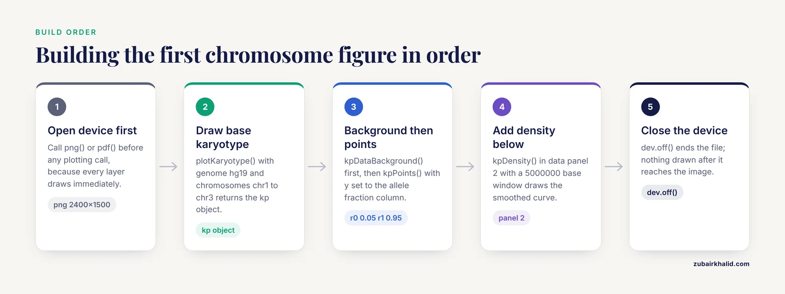
To keep the tutorial self-contained and offline, simulate a variant set against three human chromosomes. GRanges is the Bioconductor container for genomic intervals, holding chromosome names, starts, ends, and any metadata columns. toGRanges() from regioneR converts data frames or files into GRanges.
library(karyoploteR)
library(regioneR)

set.seed(42)

chr_len <- c(chr1 = 249250621, chr2 = 242193529, chr3 = 198022430)

make_variants <- function(chr, len, n) {
  pos <- sort(sample.int(len, n))
  toGRanges(data.frame(chr = chr, start = pos, end = pos,
                       af = round(runif(n), 2)))
}

variants <- c(
  make_variants("chr1", chr_len["chr1"], 120),
  make_variants("chr2", chr_len["chr2"], 120),
  make_variants("chr3", chr_len["chr3"], 120)
)
The chromosome lengths are the standard GRCh37 values for chr1, chr2, and chr3. The af column simulates an allele fraction, the fraction of reads carrying the alternate allele, which runs from 0 to 1. Inspect the result:
head(variants)You should see a GRanges object with seqnames, ranges, and one metadata column named af. Exact positions depend on the seed and R version, but the structure looks like this:
GRanges object with 6 ranges and 1 metadata column:
    seqnames    ranges strand |        af
       <Rle> <IRanges>  <Rle> | <numeric>
  [1]     chr1   1051392      * |      0.41
  [6]     chr1   2345678      * |      0.87
  [7]     chr1   3456789      * |      0.05
  [4]     chr1   4567890      * |      0.62
  [8]     chr1   5678901      * |      0.33
  [9]     chr1   6789012      * |      0.74
Step 2: Draw the base karyotype
kp <- plotKaryotype(genome = "hg19", chromosomes = c("chr1", "chr2", "chr3"))The plotting window now shows three horizontal ideograms with cytoband shading and chromosome names on the left. Omit the chromosomes argument and every chromosome in the genome appears, including chrX and chrM. hg19 is the UCSC-style name for GRCh37, and the built-in genome layouts use chr-prefixed names. The kp object records where each chromosome and base sits on the device, which is exactly what the overlay functions consult.
Step 3: Add a points track
kpDataBackground(kp, data.panel = 1, color = "#EEEEEE")
kpPoints(kp, data = variants, y = variants$af,
         r0 = 0.05, r1 = 0.95, pch = 16, cex = 0.5, col = "#2166AC")
A light gray strip appears above each ideogram, and 360 blue points scatter across the three strips. Each point sits horizontally at its genomic position and vertically at its allele fraction, which works directly because af already runs from 0 to 1. For any other measurement, rescale first:
y <- (x - min(x)) / (max(x) - min(x))The pch and cex arguments are standard base graphics settings for point character and size.
Step 4: Add a second track below the chromosomes
kpDataBackground(kp, data.panel = 2, color = "#F7F7F7")
kpDensity(kp, data = variants, window.length = 5000000,
          r0 = 0, r1 = 1, data.panel = 2, col = "#B2182B")
kpDensity slides a 5 megabase window across each chromosome and draws the smoothed density of variant positions as a red curve below each ideogram. Peaks mark clusters. window.length is in bases.
Step 5: Stack two tracks in one panel with autotrack
Panels are not the only way to separate data types. autotrack(i, n) returns the r0 and r1 values that carve track i out of n equal slots with a small gap between them, and that arithmetic is the backbone of every multi-track figure:
kp <- plotKaryotype(genome = "hg19", chromosomes = c("chr1", "chr2", "chr3"))

t1 <- autotrack(1, 2)
t2 <- autotrack(2, 2)

kpPoints(kp, data = variants, y = variants$af,
         r0 = t1$r0, r1 = t1$r1, data.panel = 1,
         pch = 16, cex = 0.5, col = "#2166AC")
kpDensity(kp, data = variants, window.length = 5000000,
          r0 = t2$r0, r1 = t2$r1, data.panel = 1, col = "#B2182B")
Both tracks now share the upper panel, points on top and density below. Change the 2 to 5 and you get five labeled slots ready for five data types.
Step 6: Add markers, base numbers, and band labels
kp <- plotKaryotype(genome = "hg19", chromosomes = c("chr1", "chr2", "chr3"))

genes <- toGRanges(data.frame(
  chr   = c("chr1", "chr2", "chr3"),
  start = c(150000000, 90000000, 88000000),
  end   = c(150400000, 90400000, 88400000)
))

kpPlotMarkers(kp, data = genes, labels = c("GENEA", "GENEB", "GENEC"))
kpAddBaseNumbers(kp, tick.dist = 50000000, minor.tick.dist = 10000000,
                 add.units = TRUE)
kpAddCytobandLabels(kp, cex = 0.4)
kpPlotMarkers draws a leader line from each interval to its label, and long gene names can be rotated with its text.orientation option. kpAddBaseNumbers places major ticks every 50 megabases and minor ticks every 10 megabases, with add.units=TRUE appending Mb to the numbers. kpAddCytobandLabels writes band names on the ideograms, which becomes readable once cex drops to roughly 0.4. In a combined figure, give markers their own autotrack slot so they never collide with your data tracks.
Step 7: Zoom into a locus
kpz <- plotKaryotype(genome = "hg19",
                     zoom = toGRanges("chr1:100000000-150000000"))
kpDataBackground(kpz, data.panel = 1)
kpPoints(kpz, data = variants, y = variants$af,
         r0 = 0.05, r1 = 0.95, pch = 16, cex = 0.7, col = "#2166AC")
kpAddBaseNumbers(kpz, tick.dist = 5000000, minor.tick.dist = 1000000,
                 add.units = TRUE)
The figure now shows only chr1 from 100,000,000 to 150,000,000, stretched across the full width, with ticks every 5 megabases. The same variants object works unchanged because karyoploteR recomputes the coordinate mapping and ignores data outside the window.
Step 8: Export the figure
Because every call draws immediately, the export device must be open before the first plotting call:
png("karyoplot.png", width = 2400, height = 1500, res = 220)

kp <- plotKaryotype(genome = "hg19", chromosomes = c("chr1", "chr2", "chr3"))
kpDataBackground(kp, data.panel = 1, color = "#EEEEEE")
kpPoints(kp, data = variants, y = variants$af,
         r0 = 0.05, r1 = 0.95, pch = 16, cex = 0.5, col = "#2166AC")

dev.off()
At 220 pixels per inch, a 2400 by 1500 pixel canvas prints about 10.9 by 6.8 inches. For vector output, swap png() for pdf("karyoplot.pdf", width = 11, height = 7), where width and height are in inches. Vector PDFs stay sharp at any magnification and are the safer submission format for journals.
Loading Real Genomic Data Formats
Simulated data proves the API. Real analysis needs converters, and the pattern is always the same: get your features into a GRanges whose chromosome names match the plot, then call any kp function.
VCF files
A VCF (variant call format) file stores SNVs and indels with a chromosome, a position, and per-sample genotypes. The vcfR package reads compressed VCFs directly:
library(vcfR)

vcf <- read.vcfR("cohort.variants.vcf.gz")
fix <- as.data.frame(getFIX(vcf))

var_gr <- toGRanges(data.frame(chr = fix$CHROM,
                               start = as.numeric(fix$POS),
                               end   = as.numeric(fix$POS)))
getFIX() extracts the fixed columns (CHROM, POS, ID, REF, ALT, QUAL, FILTER). If the VCF uses Ensembl-style names (1, 2, X) and you plotted a chr-prefixed genome, harmonize them before plotting:
library(GenomeInfoDb)
seqlevelsStyle(var_gr) <- "UCSC"
VariantAnnotation::readVcf is the Bioconductor-native alternative when you also need genotype fields, and both routes end in the same place, a GRanges handed to kpPoints or kpPlotRegions. Colleagues who prefer interfaces over scripts can review the same VCFs interactively with tools built for that purpose, such as XVCF, which was designed to summarize and visualize VCF data without command-line work [3].
BED and other interval files
BED files are tab-delimited chromosome, start, end tables, and toGRanges() reads them directly:
peaks <- toGRanges("macs2_peaks.bed")For any other tabular format, read it with read.table or read.delim, name the first three columns chr, start, and end, and pass the data frame to toGRanges(). The multi-format problem is well trodden in R. LDblockR, for example, ingests VCF, HapMap, and PLINK genotype formats in pure R before its linkage disequilibrium calculations and regional plots [4].
BAM coverage and bigWig scores
A BAM file is the standard aligned-read container, and a bigWig file stores a continuous per-base signal such as coverage or conservation. karyoploteR has dedicated overlay functions for both:
kp <- plotKaryotype(genome = "hg19",
                    zoom = toGRanges("chr7:55000000-56000000"))
kpPlotBAMCoverage(kp, data = "tumor.sorted.bam")
kp <- plotKaryotype(genome = "hg19")
kpPlotBigWig(kp, data = "chipseq_signal.bw")kpPlotBAMCoverage needs the BAM index (the .bai file) sitting next to the BAM, and both functions behave best inside a zoom, because whole-genome per-base coverage overwhelms a chromosome-scale axis. For full control, import the bigWig with rtracklayer::import(), which returns a GRanges with a score column, and draw it yourself with kpLines.
The same pattern scales into pipelines. Automated genomics suites embed R-based visualization steps exactly this way, and CGAS, a chloroplast genome analysis pipeline, wires R graphics into its workflow as a concrete example of moving from raw data to finished figures without manual steps [6]. Wrap the plotting block of this tutorial in a function that takes a GRanges and a file name, and you have the same capability for your own project.
Custom Genomes: Yeast, Non-Model Organisms, and Draft Assemblies
Built-in chromosome layouts cover a set of standard genomes, including hg38, hg19, mm10, mm9, rn6, dm6, and ce11. Everything else, from baker's yeast to a newly assembled crop line, takes one of two routes.
The first route is a custom genome, which is just a GRanges or data frame of chromosome names and lengths. Here is Saccharomyces cerevisiae, the yeast used in the yEvo classroom evolution experiments, with nuclear chromosome lengths from the sacCer3 assembly (the first six chromosomes, extend the vector through chrXVI):
sc_genome <- toGRanges(data.frame(
  chr   = c("chrI", "chrII", "chrIII", "chrIV", "chrV", "chrVI"),
  start = rep(1, 6),
  end   = c(230218, 813184, 316620, 1531919, 576874, 270161)
))

kp <- plotKaryotype(custom.genome = sc_genome)
Six plain boxes appear, one per chromosome, because custom genomes have no cytobands unless you supply a band table through the cytobands argument. Overlaying data works exactly as before:
muts <- toGRanges(data.frame(
  chr   = c("chrI", "chrII", "chrIII", "chrIV", "chrV", "chrVI"),
  start = c(120445, 451233, 240987, 1102456, 300122, 150033),
  end   = c(120445, 451233, 240987, 1102456, 300122, 150033)
))

kpPlotMarkers(kp, data = muts, labels = paste0("mut", seq_along(muts)))
That figure, mutations pinned to yeast chromosomes, is the static cousin of the interactive chromosome map at the center of the yEvo Mutation Browser, which was built in R Shiny to help students interpret whole-genome sequencing of evolved yeast lines [1].
The second route is a BSgenome package, the Bioconductor containers that hold full genome sequences. Install the one matching your assembly, read its chromosome lengths, and build the same custom genome without hardcoding numbers:
BiocManager::install("BSgenome.Scerevisiae.UCSC.sacCer3")
library(BSgenome.Scerevisiae.UCSC.sacCer3)

sl <- seqlengths(Scerevisiae)
sc_genome <- toGRanges(data.frame(chr = names(sl),
                                  start = 1,
                                  end = as.vector(sl)))
For draft assemblies with hundreds of contigs, pass a subset with the chromosomes argument or filter the custom genome down to the largest scaffolds. A karyotype with 400 tiny boxes communicates nothing.
Styling Tips for Multi-Track, Publication-Ready Figures
These karyoploteR tutorial tips cover the difference between a working plot and a figure a reviewer accepts.
Reserve space deliberately. Heights and margins live in the plot parameter list:
pp <- getDefaultPlotParams(plot.type = 1)
pp$ideogramheight <- 40
pp$data1height   <- 300
pp$topmargin     <- 40
pp$bottommargin  <- 40

kp <- plotKaryotype(genome = "hg19", plot.params = pp)
data1height controls the height of data panel 1 and ideogramheight the chromosome strip. The units are relative and respond to trial and error, so iterate on screen before exporting.
Map values to color. Color vectors recycle across the data, so categorical coloring is one line:
variants$class <- sample(c("SNV", "indel"), length(variants), replace = TRUE)

kpPoints(kp, data = variants, y = variants$af,
         col = ifelse(variants$class == "SNV", "#2166AC", "#B2182B"),
         r0 = 0.05, r1 = 0.95, pch = 16, cex = 0.5)
Pick colorblind-safe palettes and keep the same color meaning across every panel of a multi-figure document.
Label every track. Unlabeled strips force readers to guess:
kpAddLabels(kp, labels = "Allele fraction", r0 = 0.05, r1 = 0.95,
            data.panel = 1, cex = 0.8)
Give the figure a title.
kpAddMainTitle(kp, main = "Variant distribution, cohort A")The base graphics title() function also works if you prefer it.
Compose, do not cram. A chromosome-scale karyoploteR panel pairs well with locus-level ggplot2 figures in a larger layout, which matches
Finishing the Styling Toolkit: Composing Panels, Legends, and Fine-Grained Labels
A chromosome-scale karyoploteR panel pairs well with locus-level ggplot2 figures in a larger layout, which matches the way published cancer genomics figures are actually assembled: summary plots in ggplot2, annotation helpers such as ggrepel, and data reshaping in dplyr and tidyr [2]. The practical way to combine them is to draw the karyoploteR panel first into its own file, or to place both onto a shared page with base R's layout() or the grid and cowplot ecosystems. Because karyoploteR draws immediately onto the current device in base-graphics style, a layout matrix that reserves a row or column for the karyotype works with no special adapters:
png("combined.png", width = 3000, height = 2000, res = 220)
layout(matrix(c(1, 2), nrow = 2), heights = c(1, 2))

kp <- plotKaryotype(genome = "hg19", chromosomes = c("chr1", "chr2", "chr3"))
kpDataBackground(kp, data.panel = 1, color = "#EEEEEE")
kpPoints(kp, data = variants, y = variants$af,
         r0 = 0.05, r1 = 0.95, pch = 16, cex = 0.5, col = "#2166AC")

par(mar = c(5, 4, 2, 2))
plot(af_locus_df$pos, af_locus_df$af, pch = 16,
     xlab = "Position on chr1 (Mb)", ylab = "Allele fraction")
dev.off()
The same immediate-drawing behavior makes legends straightforward. karyoploteR's plotting region runs from 0 to 1 in both directions in base-graphics coordinates, so the standard legend() function lands where you expect it:
legend("topright",
       legend = c("SNV", "indel"),
       col = c("#2166AC", "#B2182B"),
       pch = 16, cex = 0.8, bty = "n")
If a legend overlaps data, shift it by passing explicit x and y coordinates between 0 and 1, or shrink the r1 of your topmost track so a margin is free. For per-point text, kpText() mirrors kpPoints() and takes a labels argument; for horizontal or vertical reference lines at genomic positions, kpAbline() draws them relative to the same coordinate mapping as everything else. Two rules keep fine-grained labels readable at manuscript scale: drop cex well below what looks right on screen, because a 220 dpi export magnifies everything, and prefer kpAddLabels() for track names over ad hoc text() calls, since kpAddLabels() already understands the r0 to r1 geometry of the panel it labels.
A Second Worked Example: Copy-Number Segments, Step by Step
Copy-number data exercises a different part of the API than single-nucleotide variants. A copy-number segment is an interval, not a point, so it needs kpRect() or kpSegments() rather than kpPoints(), and the copy-number value is a measurement that must be normalized before it maps to height.
Start from a simulated segment table, the shape of what CBS or similar segmentation tools emit:
set.seed(7)

cn_segments <- toGRanges(data.frame(
  chr = sample(c("chr1", "chr2", "chr3"), 60, replace = TRUE),
  start = sample.int(150000000, 60),
  cn = sample(0:6, 60, replace = TRUE)
))
end(seg_sorted) <- seg_sorted$cn
cn_segments <- sort(cn_segments)
end(cn_segments) <- end(cn_segments) + 5000000
In real analysis you would keep the true segment ends; here fixed 5 megabase widths keep the simulation honest about what matters, which is the mapping of intervals and values. Normalize copy number to the 0 to 1 range that the y argument expects. With states from 0 to 6, dividing by the maximum works:
cn_segments$y <- cn_segments$cn / max(cn_segments$cn)Now draw segments as vertical bars whose heights encode copy number, with the ideograms between two data panels:
kp <- plotKaryotype(genome = "hg19",
                    chromosomes = c("chr1", "chr2", "chr3"),
                    plot.type = 4)

cn_cols <- c("#2166AC", "#92C5DE", "#F7F7F7",
             "#FDDBC7", "#F4A582", "#D6604D", "#B2182B")

kpDataBackground(kp, color = "#FAFAFA")
kpSegments(kp, data = cn_segments, r0 = 0.05, r1 = 0.95,
           y0 = 0, y1 = cn_segments$y,
           col = cn_cols[cn_segments$cn + 1], lwd = 3)
kpAddLabels(kp, labels = "Copy number", r0 = 0.05, r1 = 0.95, cex = 0.8)
kpAddBaseNumbers(kp, tick.dist = 50000000, minor.tick.dist = 10000000,
                 add.units = TRUE)
plot.type 4 places ideograms at the top with all data below, which is the conventional look for copy-number profiles. kpSegments() takes y0 and y1 separately, so each bar rises from the panel floor to its normalized value. The color vector is indexed directly by state, which is the simplest robust way to keep colors consistent: build the palette once at the top of the script and index it everywhere.
For broad alterations such as whole-arm gains and losses, filled bands often communicate better than bars. kpRect() paints each interval edge to edge, and a state-coded palette turns the figure into something a cytogeneticist can parse at a glance:
arm_events <- cn_segments[cn_segments$cn %in% c(0, 1, 6)]
kpRect(kp, data = arm_events, r0 = 0.05, r1 = 0.30,
       col = ifelse(arm_events$cn < 2, "#2166AC", "#B2182B"),
       border = NA)
Losses in blue, gains in red, at a fixed shallow band near the ideogram. This two-layer pattern, bars for graded values plus rects for categorical calls, is the workhorse composition for tumor copy-number figures.
A Third Worked Example: A Multi-Sample, Multi-Track Figure with autotrack
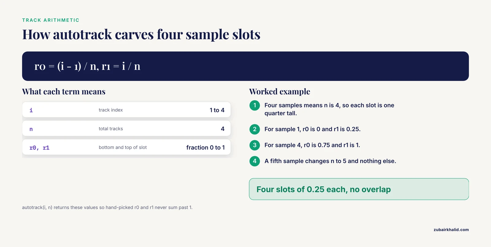
The most common publication request is the same plot repeated across samples: eight tumors, twelve evolved clones, five tissues. autotrack() plus a loop is the entire trick, and writing it out once means you never hand-compute r0 and r1 again.
Build simulated data for four samples, each a GRanges of variant positions:
set.seed(11)

sample_names <- c("tumorA", "tumorB", "tumorC", "tumorD")
sample_vars <- lapply(seq_along(sample_names), function(i) {
  pos <- sort(sample.int(249250621, 40))
  toGRanges(data.frame(chr = "chr1",
                       start = pos, end = pos))
})
names(sample_vars) <- sample_names
Now carve data panel 1 into four slots, one per sample, and draw each one. The loop index drives autotrack, so adding a fifth sample means changing one number in total.tracks:
png("multisample.png", width = 2600, height = 1400, res = 220)

kp <- plotKaryotype(genome = "hg19", chromosomes = "chr1")

n <- length(sample_vars)
track_colors <- c("#2166AC", "#B2182B", "#1B7837", "#762A83")

for (i in seq_len(n)) {
  at <- autotrack(i, n, data.panel = 1)
  kpDataBackground(kp, data.panel = 1,
                   r0 = at$r0, r1 = at$r1,
                   color = "#F5F5F5", border = NA)
  kpPoints(kp, data = sample_vars[[i]],
           y = runif(length(sample_vars[[i]])),
           r0 = at$r0, r1 = at$r1, data.panel = 1,
           pch = 16, cex = 0.4, col = track_colors[i])
  kpAddLabels(kp, labels = sample_names[i],
              r0 = at$r0, r1 = at$r1, data.panel = 1, cex = 0.7)
}

dev.off()
Three details deserve attention. First, kpDataBackground() accepts r0 and r1, so each sample's background strip matches its track exactly, and border = NA keeps the slots from reading as a grid. Second, kpAddLabels() is called inside the loop with the same autotrack values, which is why every strip arrives pre-labeled. Third, in real code the y value would come from each sample's own measurement, normalized per sample or across the whole cohort depending on what comparison you want readers to make; normalizing per sample makes within-sample structure visible, while a shared scale makes cross-sample comparisons honest. Decide deliberately and state the choice in the figure caption.
The identical skeleton handles interval data by swapping kpPoints() for kpPlotRegions(), which stacks non-overlapping regions within its slot, and for density views by swapping it for kpDensity(). Because every variant of the figure derives from one loop, a reviewer request for six samples instead of four, or for chr2 added, is a one-line edit. This is also the natural seam where a plotting step joins an automated pipeline; workflows that wire R graphics directly into genomics pipelines, such as the CGAS chloroplast genome analysis suite, rely on exactly this kind of parameterized plotting block [6].
Common Mistakes in karyoploteR and How to Fix Them
These are the failures that account for most frustration in a first week with the package, in rough order of frequency.
Chromosome name mismatch. Your data says 1 and the plot says chr1, or your data says chrI while the genome layout says chr1. Nothing errors; the points simply never appear. Diagnose it directly:
unique(as.character(seqnames(variants)))Compare that output against the chromosome names visible in the plot. Fix with seqlevelsStyle() from GenomeInfoDb when the styles are known, or with a simple prefix edit when they are not. This single mistake explains a large share of empty karyoploteR figures.
Drawing outside the device lifetime. Because every kp function draws immediately, calling kpPoints() after dev.off() throws an error, and calling plotKaryotype() before opening the file device sends the figure to the screen viewer at screen resolution. Keep the pattern strict: open the device, plot, close the device, in that order, inside one block.
Background drawn after data. kpDataBackground() is a filled rectangle, and layers stack in call order. If it is called after kpPoints(), it paints over them. Backgrounds go first.
The y argument outside 0 to 1. Raw p-values, read depths, or fold changes passed directly to y are silently clipped or flattened to one edge of the track. Normalize first, and if the result looks suspicious, print range(y) before plotting.
Expecting ggplot2 semantics. There is no + operator, no aes(), and no automatic legend. The kp object is not a data structure you mutate; it is a drawing context. Reads of the code go more smoothly once you treat each kp call as a paint command.
Whole-genome per-base draws. kpPlotBAMCoverage() across an entire chromosome or genome produces an unreadable solid block and wastes time. Per-base coverage belongs in a zoom; genome-wide questions about coverage belong in kpDensity() over a wide window or in bigWig scores aggregated with rtracklayer before drawing.
A missing BAM index. kpPlotBAMCoverage() reads the .bai companion and fails without it. Index the BAM with your aligner or samtools index before plotting, and confirm the two files sit in the same directory with matching names.
Cytoband requests on a custom genome. kpAddCytobandLabels() has nothing to write unless a band table was supplied through the cytobands argument of plotKaryotype(). For custom genomes, either skip band labels or provide the table.
Unnormalized multi-track heights. Stacking four tracks with hand-picked r0 and r1 values that sum to more than 1 pushes the last track off the panel or into the ideograms. autotrack() exists precisely to prevent this; use it whenever track count can change.
Forgetting the chromosomes argument on built-in genomes. A quick test against hg19 draws all 24 chromosomes, each a sliver, and the figure looks broken. Pass chromosomes = even during exploration.
Troubleshooting a Broken Figure: A Diagnostic Sequence
When a figure comes out wrong, resist the urge to tweak parameters randomly. Work down this sequence, which isolates the failure layer by layer.
Step 1: Does the bare karyotype draw?
kp <- plotKaryotype(genome = "hg19", chromosomes = "chr1")If this fails, the problem is installation, the genome name, or the graphics device, not your data. Check packageVersion("karyoploteR") and try a fresh device.
Step 2: Do the chromosome names match? Print unique(seqnames(data)) and compare character by character against the labels on the ideograms. Case and prefix both matter.
Step 3: Are the coordinates inside the plotted chromosomes? Features beyond the end of a chromosome are clipped silently by default. Compare max(end(gr)) against the chromosome length in the genome layout, and for custom genomes confirm every interval fits inside the lengths you supplied.
Step 4: Is y in range and finite? summary(y) catches NA values, infinities from a divide-by-zero in normalization, and out-of-range values in one line. NA values in y produce missing points, which often read as data loss when they are data formatting.
Step 5: Is the track geometry what you intended? Temporarily draw kpDataBackground() with the same r0 and r1 as the suspect track. If the background appears where the data should, the geometry is correct and the data mapping is the problem; if the background appears in the wrong place, fix r0 and r1 before touching anything else.
Step 6: Rebuild in order. Comment out every call after plotKaryotype() and re-add them one at a time. The first call where the figure changes unexpectedly is the faulty layer, and in most sessions that takes under two minutes.
This layered diagnosis mirrors a broader principle in genomics tooling: failures compound across steps, so isolating one layer at a time is the reliable route to a fix, and fragmented toolchains without scripted intermediate checks are a documented source of hard-to-trace provenance problems [5]. A plotting script is small enough that the discipline costs almost nothing.
Common Misconceptions About karyoploteR
Misconception: karyoploteR will scale my data for me. The r0 to r1 system describes where a track lives, not how values map into it. Every y you pass to kpPoints(), kpLines(), or kpSegments() should already run from 0 to 1. The package scales your y into the track window, which is a different operation from normalizing raw measurements.
Misconception: zoom mutates the data. The zoom argument of plotKaryotype() changes only the visible window and the coordinate mapping. The GRanges you pass is untouched, data outside the window is ignored, and the same object can feed both a genome-wide plot and a zoomed plot in the same script.
Misconception: panel 1 and panel 2 are the same thing drawn in different places. They are independent drawing surfaces with independent r0 to r1 systems. Track geometry set for one does not transfer to the other, and forgetting the data.panel argument is a classic way to draw a track in an unexpected strip, which is why explicitly passing data.panel in every call is a reasonable habit even when the default would be correct.
Misconception: a custom genome requires a cytoband file. A cytoband table is optional decoration. A two-column table of chromosome names and lengths produces a perfectly serviceable karyotype of plain boxes, which is the standard look for non-model organisms and draft assemblies.
Misconception: karyoploteR replaces a genome browser. It is a figure factory, not an explorer. The division of labor is real: browsers win for interactive scrolling and base-resolution questions, and scripted chromosome maps win for reproducible, publication-oriented overviews, the same division that motivates pairing interactive VCF review tools such as XVCF with scripted summarization [3].
Misconception: kp functions return useful data objects. They return the kp drawing context, or nothing. Computation belongs upstream in GenomicRanges and regioneR; karyoploteR is the presentation layer.
How karyoploteR Compares with ggplot2, Genome Browsers, and Other Figure Styles
Choosing a plotting tool is easier when you are honest about what each one is for.
karyoploteR versus ggplot2. ggplot2 maps data to abstract axes and is unbeatable for distributions, regression summaries, and locus-level detail. Its weakness for chromosome figures is structural: the x axis is a number line, and the chromosome, with its bands and centromere, is an annotation you have to fake. karyoploteR inverts that. The chromosome is the primary axis, drawn to true physical scale with cytobands, and your data is the annotation. The two compose rather than compete, and the ggplot2-plus-helpers pipeline is a documented pattern in published genomics figures [2]. A sensible split: chromosome-scale overviews in karyoploteR, per-locus detail panels in ggplot2, both driven by the same GRanges objects.
karyoploteR versus genome browsers. A browser is interactive, optimized for human exploration, and excellent at base-resolution views with rich track formats. It is poor at producing a scripted, deterministic figure with exactly the layout you specify. karyoploteR is the opposite: nothing to click, everything to script. If the deliverable is a decision made by a human exploring data, browse. If the deliverable is a PDF in a thesis or paper, plot.
karyoploteR versus interactive Shiny tools. Shiny applications occupy the middle ground, wrapping R computation in a point-and-click interface. The yEvo Mutation Browser, for example, places mutations from evolved yeast populations on a chromosome map so students can explore interactively [1], and XVCF does the analogous job for VCF review [3]. Those tools and karyoploteR figures serve different moments in the same project: Shiny for exploration and teaching, karyoploteR for the fixed artifact.
karyoploteR versus circular layouts. Circos-style circular plots excel at showing relationships between chromosomes, such as translocations and shared haplotypes, because both endpoints are visible in one glyph. For everything else, linear chromosome maps are easier to read, easier to label, and map more directly to how coordinates are reported in text. Choose circular only when the inter-chromosomal relationship is the message.
karyoploteR versus hand-built interval plots. Anything karyoploteR draws could theoretically be hand-computed in base graphics or grid by mapping coordinates to device space yourself. The value of the package is that it owns the mapping, the cytobands, the tick arithmetic, and the zoom bookkeeping, which is the same argument made for purpose-built integration packages elsewhere in R genomics, where LDblockR ingests standard genotype formats and produces regional plots natively rather than leaving users to assemble the plumbing [4].
Practical Applications Across Domains
The API is small, which means the same three compositions cover most real use cases.
Variant distribution overviews. Points at variant positions, colored by class or consequence, with a density curve underneath to reveal clustering. This is the tutorial figure of this article, and it serves clinical variant summaries, evolved-clone comparisons, and population screens alike. The chromosome map form has proven effective in teaching contexts precisely because position on the chromosome is intuitive in a way a table of coordinates is not [1].
Copy-number and structural-variant profiles. The segments example above generalizes directly to real tumor data: state-coded bands for calls, height-coded bars for graded copy number, and per-sample autotrack slots for cohort figures.
ChIP-seq and ATAC-seq peak landscapes. Peaks as kpPlotRegions() or kpRect() in one slot, the bigWig signal as kpPlotBigWig() or an rtracklayer-imported kpLines() track in another, and kpDensity() of peak positions genome-wide to show where binding concentrates. Importing the bigWig yourself gives you the option to summarize into fixed-width bins first, which is usually the right move at chromosome scale.
QTL and GWAS mapping. Points at marker positions with y set to a normalized statistic, markers of interest drawn with kpPlotMarkers() and leader lines, and one track per trait or per environment. The figure reads as a map of where signal lives, which is the first question any mapping project asks.
Non-model and emerging organisms. A custom genome from assembly lengths, no cytobands, and markers or density tracks on top is often the first publication figure of a new assembly. For chloroplast, mitochondrial, and other small genomes, the same code produces clean circular-adjacent overviews in linear form, and scripted generation is what allows a pipeline to regenerate the figure when the assembly or annotation changes [6].
Multi-page reports. Because every figure is a function call, generating one chromosome map per sample, per chromosome, or per analysis date is a loop, not a session of manual clicking, and each page inherits identical styling.
Working with Large Data: Downsampling, Windows, and Honest Density
Chromosome-scale axes cannot render millions of features individually, and pretending otherwise produces figures that are both slow and uninformative. Three strategies, in order of preference.
Aggregate before plotting. kpDensity() is built for this: it slides a window of window.length bases across each chromosome and counts how many features fall in each window. For 2 million SNVs across hg19, a 1 to 5 megabase window produces a smooth, readable curve where the point plot would be a solid bar. Window choice is an analysis decision, not a cosmetic one; wider windows smooth away local structure, narrower windows preserve it at the cost of noise, and stating the window in the caption lets readers judge.
Downsample deliberately. When individual marks must remain visible, sample the GRanges before plotting and disclose the sampling. A stratified approach, keeping all high-value features plus a random fraction of the rest, preserves the biologically interesting tail while keeping the draw manageable.
Summarize continuous tracks yourself. For bigWig signals at genome scale, import with rtracklayer, aggregate the score column into bins with standard GenomicRanges operations, and draw the binned means with kpLines(). This keeps the plotting function's workload proportional to the number of bins, not the number of bases, and gives you explicit control over what the figure claims the data shows.
One caution applies to all three: aggregation can manufacture or destroy apparent clustering depending on window placement and genome gaps, so sanity-check any striking density peak against the underlying intervals before writing it into a results section. Uncorrected segments of the genome with unusual mappability or repeat content will show up in density plots of raw variant calls, and a figure that invites a biological interpretation of an artifact is worse than no figure.
Turning the Tutorial into a Reusable Function and a Reproducible Pipeline
A plotting block becomes project infrastructure the moment it is parameterized. Wrap the whole figure in one function with an output path and a GRanges argument:
plot_variant_map <- function(var_gr, out_png,
                             genome = "hg19",
                             chroms = c("chr1", "chr2", "chr3")) {
  png(out_png, width = 2400, height = 1500, res = 220)
  on.exit(dev.off())

  kp <- plotKaryotype(genome = genome, chromosomes = chroms)
  kpDataBackground(kp, data.panel = 1, color = "#EEEEEE")
  kpPoints(kp, data = var_gr, y = var_gr$af,
           r0 = 0.05, r1 = 0.95, pch = 16, cex = 0.5,
           col = "#2166AC")
  kpAddMainTitle(kp, main = paste("Variants:", basename(out_png)))
  invisible(kp)
}
on.exit(dev.off()) closes the device even if a later plotting call errors, which prevents the half-open-device states that corrupt subsequent figures in a session. With this function in place, every figure in a project is one call with recorded arguments, and the entire figure, from file import through dev.off(), lives inside one script, which is the single strongest habit for keeping visualization reproducible in genomics workflows [5].
For projects that regenerate figures automatically, add three guards inside the function: verify that seqnames levels of the input intersect the plotted chromosomes and stop with an informative message if not, verify that y exists and runs between 0 and 1 before drawing, and return the kp object invisibly so callers can add layers afterward without redrawing. Ten lines of validation convert a silent empty figure into an error message that names the problem.
Per-chromosome zoom pages follow the same pattern with a loop over regions:
regions <- toGRanges(data.frame(
  chr = c("chr1", "chr2", "chr3"),
  start = c(1, 1, 1),
  end = c(249250621, 242193529, 198022430)
))

for (i in seq_along(regions)) {
  out <- sprintf("zoom_%s.png", as.character(seqnames(regions[i])))
  png(out, width = 2400, height = 900, res = 220)
  kpz <- plotKaryotype(genome = "hg19", zoom = regions[i])
  kpDataBackground(kpz, data.panel = 1)
  kpPoints(kpz, data = variants, y = variants$af,
           r0 = 0.05, r1 = 0.95, pch = 16, cex = 0.7, col = "#2166AC")
  kpAddBaseNumbers(kpz, tick.dist = 20000000,
                   minor.tick.dist = 5000000, add.units = TRUE)
  dev.off()
}
Tick spacing scales with the window: 50 megabase ticks suit a whole-chromosome view, and the zoom loop uses proportionally finer ticks so every exported page carries interpretable position labels. Close each figure with sessionInfo() recorded to a side file in scripted runs, so the exact package versions behind every exported image are recoverable months later.
A Pre-Submission Checklist for Chromosome Figures
Before any karyoploteR figure leaves your hands, walk this list.
- Names harmonized. Chromosome naming style matches between the genome layout and every data object, verified by printing seqnames levels, not by eyeballing the plot.
- Scale stated. Base-number ticks present with units, or an explicit statement in the caption that axes are schematic for custom genomes without to-scale drawing.
- Every track labeled. kpAddLabels() on each autotrack slot, no unlabeled strips anywhere in the figure.
- Colors defined and consistent. Categorical palettes colorblind-safe, identical states identically colored across all figures in the document, and the mapping stated in the caption.
- Normalization disclosed. If y values are normalized, min-max or otherwise, the caption says so, because readers will otherwise assume raw units.
- Aggregation disclosed. Density windows and downsampled points named with their parameters.
- Device matched to output. Raster exports at print-appropriate resolution, vector PDF for anything a journal may rescale, and the device opened before the first plotting call.
- Layers in deliberate order. Backgrounds first, data second, labels and reference lines last.
- Zoom windows honest. Data outside a zoomed window is absent by design, and the caption states the visible interval.
- Environment recorded. sessionInfo() output saved alongside the script, the figure regenerable from a clean session.
None of these items is specific to karyoploteR, which is the point. The package handles the chromosome geometry that generic plotting cannot, and the checklist handles the reporting discipline that no package can. Together they turn a first successful plot into a figure that survives review, and a script that survives the rerun three months later when the variant calls are updated and the figure must be regenerated exactly, with no memory of how it was made.
Sources
- The yEvo Mutation Browser: Enhancing student understanding of experimental evolution and genomics through interactive data visualization.
- Synergistic role of molecular imaging and genomics in thyroid cancer management: from diagnosis to personalized treatment.
- XVCF: Exquisite visualization of VCF data from genomic experiments.
- LDblockR: a cross-platform R toolkit for multi-format linkage disequilibrium analysis and integrated regional genomics visualization.
- SNPio: a Python interface for population genomic data processing.
- CGAS (Chloroplast Genome Analysis Suite): An automated python pipeline for comprehensive comparative chloroplast genomics.