What Is a Density Curve? Definition and Examples

By Dr. Zubair Khalid, DVM, MS, PhD · 2026-10-03

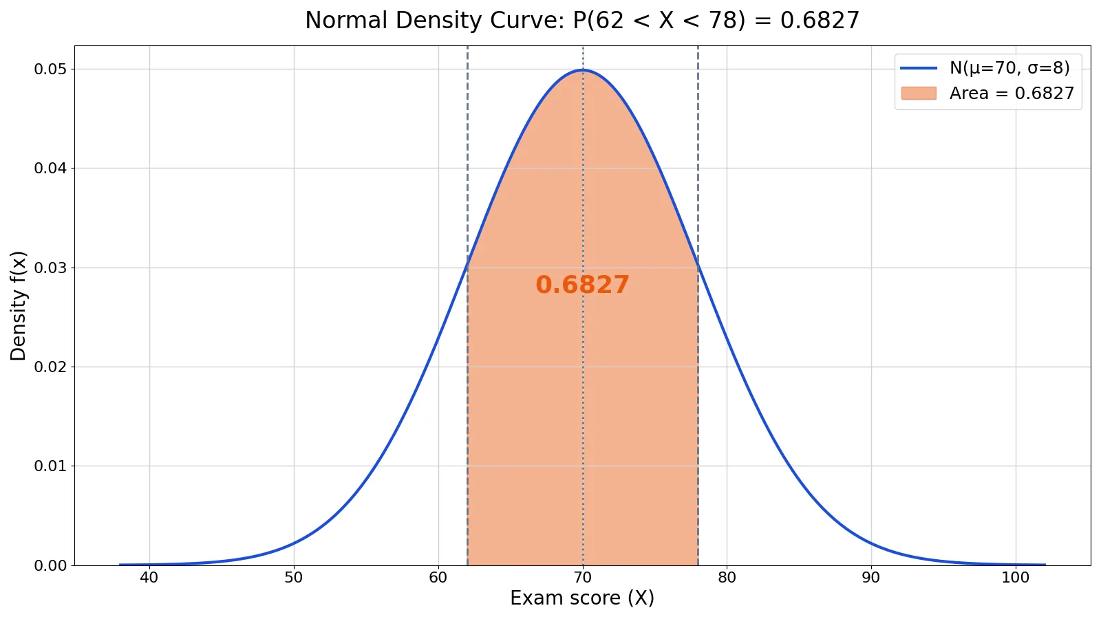
A density curve is a smooth curve that describes how probability is spread across the possible values of a continuous variable. The total area under the curve always equals 1, and the area above any range of values equals the probability of observing a value in that range. This article explains the definition, the math behind it, and how to read a density curve in practice.

Quick Answer

A density curve is an idealized model of a distribution where the area under the curve is defined to be 1 [1].
Probability comes from area, not height. The area under the curve between two values is the probability of landing between them.
The curve never goes below the horizontal axis, so density values are zero or positive.
Density curves do not have to be normal, but the normal density curve is the most widely used [1].
For a normal curve, about 68% of the total area sits within one standard deviation of the mean [1].

What a Density Curve Means

In plain terms, a density curve is a picture of a continuous distribution. Instead of listing probabilities for each separate value, it shows a smooth curve where taller regions mean values are more likely to occur and flatter regions mean they are less likely.

The precise statistical definition: a density curve is the graph of a probability density function $f(x)$ for a continuous random variable, satisfying two conditions. First, $f(x) \ge 0$ for every value of $x$. Second, the total area between the curve and the horizontal axis equals exactly 1. Because the area is 1, the curve acts as a complete probability model for the variable.

One consequence surprises many people. For a continuous variable, the probability of any single exact value is 0. You cannot ask for the probability that a measurement equals 70.000 exactly. You ask for the probability that it falls in an interval, such as between 62 and 78. That interval probability is the area under the curve over that stretch.

How It Works

The link between area and probability is written as an integral. For a continuous random variable $X$ with density $f(x)$, the probability that $X$ falls between two values $a$ and $b$ is:

$$P(a < X < b) = \int_{a}^{b} f(x)\,dx$$

Each symbol means the following.

$X$ is the continuous random variable you are measuring, such as an exam score.
$f(x)$ is the density function, the height of the curve at value $x$.
$a$ and $b$ are the lower and upper bounds of the interval you care about.
The integral sign sums the area under the curve from $a$ to $b$.

For the normal distribution, the density has a specific bell shape:

$$f(x) = \frac{1}{\sigma\sqrt{2\pi}}\, e^{-\frac{(x-\mu)^2}{2\sigma^2}}$$

Here $\mu$ is the mean, which sets the center of the curve, and $\sigma$ is the standard deviation, which sets the spread. A larger $\sigma$ produces a wider, flatter curve, and a smaller $\sigma$ produces a narrower, taller one [1]. The standard normal curve uses $\mu = 0$ and $\sigma = 1$, and its cumulative distribution function is written $\Phi(z)$.

To find an area for a normal curve, you convert your bounds to z-scores with $z = (x - \mu)/\sigma$, then read the cumulative probability from a table or a function. The area between two bounds is the difference of two cumulative probabilities.

Worked Example

Suppose a class of 10 students takes an exam, and you want the probability that a randomly chosen score falls between 62 and 78, assuming scores follow a normal distribution with mean 70 and standard deviation 8. The raw scores are shown below.

student_id	score
1	58
2	62
3	65
4	68
5	70
6	71
7	73
8	75
9	78
10	82

The steps use the assumed normal model with $\mu = 70$ and $\sigma = 8$.

Step	Value
Standardize lower bound	$z_a = (62 - 70) / 8 = -1.0000$
Standardize upper bound	$z_b = (78 - 70) / 8 = 1.0000$
CDF at lower bound	$\Phi(-1.0000) = 0.1587$
CDF at upper bound	$\Phi(1.0000) = 0.8413$
Area between bounds	$P(62 < X < 78) = 0.8413 - 0.1587 = 0.6827$

The shaded area under the curve between 62 and 78 is 0.6827, so about 68.27% of scores are expected to fall in that range. This matches the Empirical Rule, which says roughly 68% of a normal distribution lies within one standard deviation of the mean [1].

You can reproduce the result with this code.

from scipy.stats import norm
mu, sigma = 70, 8
p = norm.cdf(78, mu, sigma) - norm.cdf(62, mu, sigma)  # area between the bounds
print(round(p, 4))

Output:

0.6827

For reference, the sample mean of the 10 scores is 70.2000 and the sample standard deviation (using $n-1$) is 7.2999. Those sample values are close to the assumed model values of 70 and 8, which is why the normal curve is a reasonable stand-in here.

How to Interpret It

Reading a density curve comes down to three habits.

First, look at area, not height. A tall narrow peak and a short wide bump can cover the same total area of 1. The height only tells you relative concentration at a single point, not probability.

Second, locate the center and spread. The mean marks where the curve balances, and the standard deviation marks how far the curve stretches. On a normal curve, the points one standard deviation from the mean sit where the curve changes from bending down to bending up, called inflection points [1].

Third, shade the region you care about. If you want $P(X > 75)$, shade everything to the right of 75 and find that area. If you want $P(62 < X < 78)$, shade the middle band. The area you shade is the answer.

When to Use It (and when not to)

Use a density curve when your variable is continuous and you want probabilities over intervals. Common cases include measurement data such as heights, weights, times, temperatures, and test scores. It is also the natural tool when you want to compare a sample to a theoretical model, or when you need to compute tail probabilities for a hypothesis test or confidence interval.

Do not use a density curve for discrete counts where each value has its own probability, such as the number of heads in 10 coin flips. A bar chart or probability mass function fits that case better. You can read more about the discrete counterpart in this guide to the probability density function.

Also avoid forcing a normal curve onto data that is clearly skewed or has two peaks. A density curve can take many shapes, and the normal curve is only one option [1]. If your data is bounded between 0 and 1, such as a proportion, a beta distribution may describe it better.

Density Curve vs Histogram

A histogram and a density curve both show a distribution, but they serve different roles. The table below compares them.

Feature	Histogram	Density Curve
Source	Actual observed data	Theoretical model or smoothed estimate
Shape	Bars with gaps or touching bars	Smooth continuous line
Total area	Depends on bin width and counts	Always equals 1
Probability	Estimated from bar heights	Exact area under the curve
Best for	Exploring real samples	Computing probabilities and comparing models

A histogram with a very large sample and narrow bins starts to look like a density curve. That is the intuition behind the density curve as an idealized version of the distribution [1].

Common Mistakes

Reading the height as a probability. The fix is to always measure area over an interval, since a single point has probability 0.
Assuming every density curve is normal. The fix is to check the shape first. Skewed and bimodal data need a different curve.
Forgetting that total area must equal 1. The fix is to verify that any curve you use integrates to 1 over its full range.
Using a density curve for discrete data. The fix is to use a probability mass function or a bar chart instead.
Mixing up standard deviation and variance on the horizontal axis. The fix is to label the axis in the units of the data and mark $\mu$ and $\sigma$ clearly.
Treating the curve as exact for small samples. The fix is to remember that a fitted curve is an approximation, and small samples give unstable estimates.

Limitations

A density curve is a model, not the data itself. When you fit a normal curve to a sample, you are assuming the underlying process is normal, and that assumption can be wrong. Real data often has outliers, skew, or multiple clusters that a single smooth curve cannot capture.

The curve also cannot tell you the probability of an exact value, because that probability is always 0 for a continuous variable. And the area under the curve only gives probabilities within the model you chose. If the model is a poor fit, the areas will be misleading even though the math is correct.

Frequently Asked Questions

What does the area under a density curve represent?

The area under a density curve over a range of values equals the probability that the variable falls in that range. The total area under the entire curve is always 1, which represents 100% of all possible outcomes.

Why is the total area under a density curve equal to 1?

The area equals 1 because the curve covers every possible value the variable can take, and the sum of all probabilities must be 1. This is the same rule that applies to any valid probability distribution.

Can a density curve go above 1 on the vertical axis?

Yes. The height of a density curve is not a probability, so it can exceed 1. Only the total area is capped at 1. A narrow curve with a small spread can have a very tall peak.

What is the difference between a density curve and a probability density function?

They describe the same idea. A probability density function is the mathematical function, and the density curve is its graph. You use the function to compute areas and the curve to visualize them.

How do I find a probability from a normal density curve?

Convert your bounds to z-scores using $z = (x - \mu)/\sigma$, then find the cumulative probability for each bound. Subtract the lower cumulative probability from the upper one to get the area between them. In the worked example, that gave 0.8413 minus 0.1587, or 0.6827.

References

11.2: The Density Curve of a Normal Distribution - Mathematics LibreTexts/11%3A_Normal_Distribution/11.02%3A_The_Density_Curve_of_a_Normal_Distribution)