How to Interpret DESeq2 Results

By Dr. Zubair Khalid, DVM, MS, PhD · 2026-11-11

Interpreting DESeq2 results means reading the six-column table that the results() function returns and translating each row, one gene or transcript per row, into a defensible biological statement about effect size, uncertainty, and statistical significance. A correct interpretation answers three questions for every gene: how large is the expression change, how confident are we in that change, and how many false positives would we expect if we called everything at that threshold.

That translation matters because the DESeq2 results table is where most RNA-seq projects either succeed or quietly go wrong. DESeq2 is one of the most widely used R/Bioconductor packages for differential expression analysis of count data, and benchmarking studies place it among the strongest performers for negative binomial count data at moderate sample sizes, with better false discovery rate control, power, and stability than most alternatives when each group has six or more samples [1]. Yet the package hands you raw statistical machinery, not conclusions. Researchers who misread the fold change column, ignore the adjusted p value, or filter on the wrong quantity routinely publish gene lists that fail validation. This guide walks through the table column by column, explains the machinery that produced each number, shows a worked filtering pass, and catalogs the mistakes that trip up analysts using R for bioinformatics, whether they run DESeq2 itself or Python ports such as pyDESeq2 [2].

What Interpreting DESeq2 Results Means in Practice

When someone asks what does interpret DESeq2 results mean, the honest answer has two layers. The narrow layer is mechanical: knowing that baseMean is the average normalized count, that log2FoldChange is the effect estimate on a log2 scale, and that padj is the Benjamini-Hochberg adjusted p value. The broader layer is judgment: deciding which rows deserve attention, which numbers are trustworthy given your design and sample size, and which downstream analyses, such as pathway enrichment, will add information rather than repeat noise.

Interpretation is not a separate step bolted onto the analysis. Every choice you make upstream, including the design formula, the count import method, and the normalization strategy, changes the numbers you will later interpret. Studies of differential expression workflows show that the choice of normalization method alone can shift which genes land on the final DEG list, which is why comparative tools that aggregate results across normalization methods have been developed [3]. Interpretation therefore starts before you ever call results().

The Results Table: One Row Per Gene

Calling results(dds) on a fitted DESeqDataSet returns a DESeqResults object that prints as a table with these columns:

You can inspect the column definitions directly in R with mcols(res)$description, which is a habit worth building because it keeps the definitions attached to your actual object rather than to your memory.

baseMean: the size of the signal

baseMean is the average of the size-factor-normalized counts for that gene across every sample in the dataset, both conditions combined. It answers the question "how expressed is this gene at all." A gene with a baseMean of 2 is a whisper even if it carries an impressive fold change, because estimates for very low-count genes are unstable and are frequently filtered out before testing. A gene with a baseMean of 5,000 and a modest fold change may be far more biologically consequential than a tiny-count gene with a dramatic-looking ratio. Always read the fold change column together with the baseMean column.

log2FoldChange: the effect size

The log2FoldChange column is the log base 2 of the ratio of expression between the conditions in your contrast. A value of 1 means a doubling, a value of -1 means a halving, and a value of 0 means no modeled difference. Two details cause most of the misreadings in DESeq2 results interpretation.

First, the sign and direction depend entirely on the contrast you specified. With a factor condition where the reference level is "control", results(dds) reports log2(treated divided by control), so positive values mean higher in treated. If you instead pass contrast=c("condition", "treated", "control"), the direction is explicit regardless of factor level order. Many puzzling sign flips between collaborators come down to the contrast ordering, not to biology.

Second, the fold change is a model-based quantity. DESeq2 fits a generalized linear model with a negative binomial distribution to the counts, using a logarithmic link, so the reported fold change comes from the fitted model coefficients, not from a simple ratio of average raw counts. This is a feature, because the model borrows information across genes and accounts for the mean-variance relationship, but it means the number will not exactly reproduce a hand calculation.

lfcSE: the uncertainty

lfcSE is the standard error of the log2 fold change. Divide the fold change by this number and you get the stat column. A gene with a fold change of 4 and a standard error of 0.2 gives a statistic of about 20, an overwhelming signal. The same fold change of 4 with a standard error of 2.5 gives a statistic of 1.6, which is unimpressive. Reading the fold change without the standard error is how analysts convince themselves that small, noisy effects are real.

stat and pvalue: the Wald test

DESeq2 tests each gene by default with a Wald test, which asks whether the model coefficient for your contrast differs from zero. The stat column is the z-like statistic, and the pvalue column is its two-sided p value under a normal approximation. If you pass test="LRT" when running DESeq(), the results table instead reflects a likelihood ratio test comparing your full design against a reduced model, which is the right tool when you care about whether any of several coefficients matter, for example across a multi-level time course, rather than about a single pairwise contrast.

padj: the false discovery rate

The padj column is the column that determines most published gene lists, and it is the most misunderstood. These p values are adjusted for multiple testing using the Benjamini-Hochberg procedure. A padj of 0.03 does not mean there is a 3 percent chance this particular gene is not differentially expressed. It means that if you called every gene with padj at or below 0.03 significant, the expected proportion of false discoveries among those calls would be at most about 3 percent. Formally, the adjusted p value is the smallest false discovery rate at which the gene would be called significant.

This distinction matters at scale. A typical mammalian RNA-seq experiment tests roughly 20,000 genes. Without correction, a p value cutoff of 0.05 would be expected to flag about 1,000 genes by pure chance even in data with no true differences. The Benjamini-Hochberg procedure controls that inflation, which is why reporting unadjusted pvalue cutoffs in a DESeq2 results table is a red flag in any review.

What DESeq2 Did Before Handing You This Table

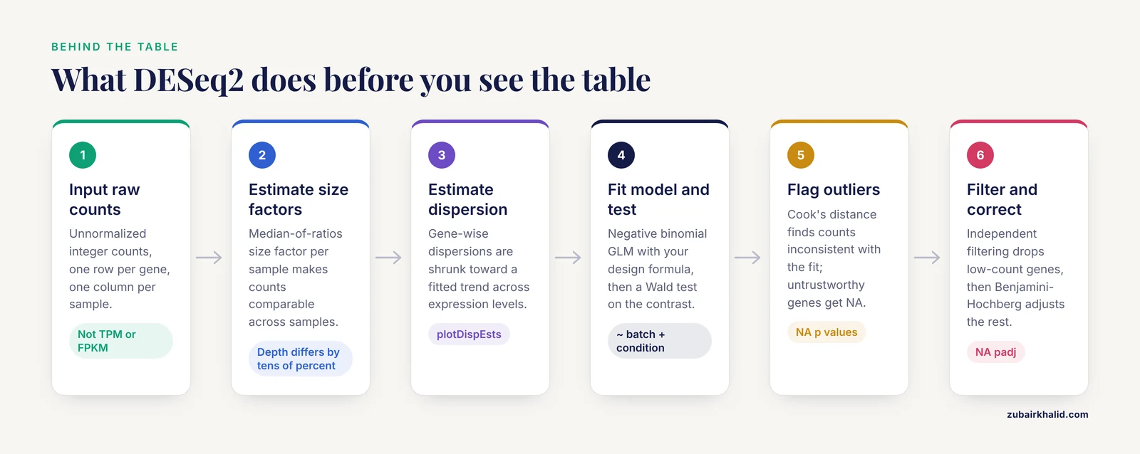
Understanding each column is easier once you know the pipeline that produced it. The steps below summarize the standard DESeq2 workflow as documented in the package and its publications.

1. Input raw counts. DESeq2 expects unnormalized integer counts, one row per gene, one column per sample, from a count matrix or from transcript quantifiers imported through tximport-style tools. In Python workflows, pytximport provides the equivalent bridge, converting transcript-level estimates from tools such as Salmon or RSEM into gene-level counts suitable for differential analysis [4]. Feeding TPM or FPKM values directly into DESeq2 is a mistake, because those quantities have already removed the information about library size and count variance that the model needs.

1. Estimate size factors. Sequencing depth differs between samples, sometimes by tens of percent. DESeq2 computes a size factor for each sample using a median-of-ratios approach so that counts become comparable across samples. These size factors are the denominator behind baseMean and normalized counts accessed with counts(dds, normalized=TRUE). Residual library-size effects after normalization remain an active research concern, with one large-scale analysis of over 100 public datasets reporting that normalized counts for a substantial proportion of genes still correlate with library size under widely used correction approaches [5]. This is a reason to check size factor spreads rather than assume the correction was perfect.

1. Estimate dispersion. In negative binomial models, dispersion describes how much a gene's counts vary beyond what Poisson noise alone would predict. DESeq2 estimates gene-wise dispersions, fits a trend across genes with similar expression levels, and then shrinks individual estimates toward that trend. The plotDispEsts function lets you eyeball whether the shrinkage behaved sensibly.

1. Fit the model and test. For each gene, DESeq2 fits a negative binomial generalized linear model with your design formula, for example ~ batch + condition, and performs a Wald test on the contrast of interest. Genes where every sample in one group has zero counts produce NA p values because the test is undefined.

1. Flag outliers. DESeq2 computes Cook's distance for each sample within each gene to detect counts that are inconsistent with the fitted model. Depending on the number of samples and coefficients, flagged counts may be replaced by trimmed values, and genes whose p values cannot be trusted because of outliers get NA values in the results.

1. Apply independent filtering and multiple testing correction. Before Benjamini-Hochberg correction, DESeq2 filters out genes with very low mean normalized counts, choosing the cutoff that maximizes the number of genes rejected at your chosen alpha. Filtered genes receive NA padj values. This filtering increases detection power for the genes that remain because fewer tests are corrected.

Automated pipelines wrap this same sequence. SeqExpressionAnalyser bundles quality control through differential expression into a single R Shiny application [6], and RNA-SeqEZPZ provides a point-and-click path from FASTQ files through differential expression and pathway analysis with either bash or Nextflow backends [7]. These tools execute the identical steps, so the interpretation rules in this article apply to their outputs as well.

Reading the Fold Change Correctly

Direction and contrasts

Write down your contrast before you open the results table. With a design of ~ condition and a two-level factor, the default contrast places the last level of the factor in the numerator. Explicit contrasts remove ambiguity:

res <- results(dds, contrast = c("condition", "treated", "control"))

For multi-level factors, interaction designs, and paired designs, the same rule applies: the Name column of the results object tells you exactly which coefficient or contrast was tested, and resultsNames(dds) lists the available coefficients. An analyst who cannot state, in one sentence, which condition is the numerator of every log2FoldChange in the table is not ready to interpret the table.

Fold change shrinkage

By default, results() reports unshrunken maximum-likelihood fold change estimates. For genes with low counts or high dispersion, these estimates can be extreme and noisy. The lfcShrink() function applies empirical Bayes shrinkage, for example with type="apeglm" or type="ashr", which pulls weakly supported fold changes toward zero while leaving strongly supported ones largely intact. Shrunk estimates are the better choice for ranking genes, for visualization, and for any statement about effect magnitude. Unshrunken estimates remain the reference for reproducibility across package versions, which is why the results object stores both conventions in recent DESeq2 releases.

Fold change thresholds

Many journals and reviewers expect a minimum effect size alongside significance. DESeq2 supports this directly through the lfcThreshold argument of results(), which shifts the null hypothesis so that genes must exceed a specified fold change threshold to reject. This test-treating approach is statistically cleaner than post hoc filtering on abs(log2FoldChange) > x, because it incorporates the threshold into the hypothesis rather than silently discarding significant genes with small effects.

A concrete published example shows how the two-stage logic works in practice. In a study of human corneal fibroblast transdifferentiation, DESeq2 analysis with an adjusted p value below 0.05 identified 3,843 differentially expressed genes and transcripts between corneal fibroblasts and myofibroblasts, and an additional filter requiring the absolute log2 fold change to be at least 1.5 narrowed the list to 816 upregulated and 739 downregulated genes, which were then carried into pathway enrichment with GSEA, PANTHER, and Reactome and network analysis with Cytoscape and cytoHubba [8]. The two-stage structure, significance first and effect size second, is a reasonable template, though using lfcThreshold within the test itself is the more defensible variant.

Reading the p-Values Correctly

pvalue versus padj

Report padj as your primary criterion and treat pvalue as a secondary diagnostic. A common and useful diagnostic is the raw p value histogram. Under a null-heavy genome, you expect a flat distribution with a spike near zero from true signals. A histogram that instead rises toward 1.0 suggests a problem, such as unmodeled batch effects, poor count modeling at low counts, or sample mislabeling.

The alpha parameter

The alpha argument of results() sets the target false discovery rate used both for the Benjamini-Hochberg correction and for the independent filtering optimization. The default is 0.10 in recent DESeq2 versions, and many analysts explicitly pass alpha=0.05 to match common reporting conventions. If your filtering and your correction disagree about alpha, your padj values and your expectations about them can drift apart, so set alpha deliberately.

Why padj contains NA values

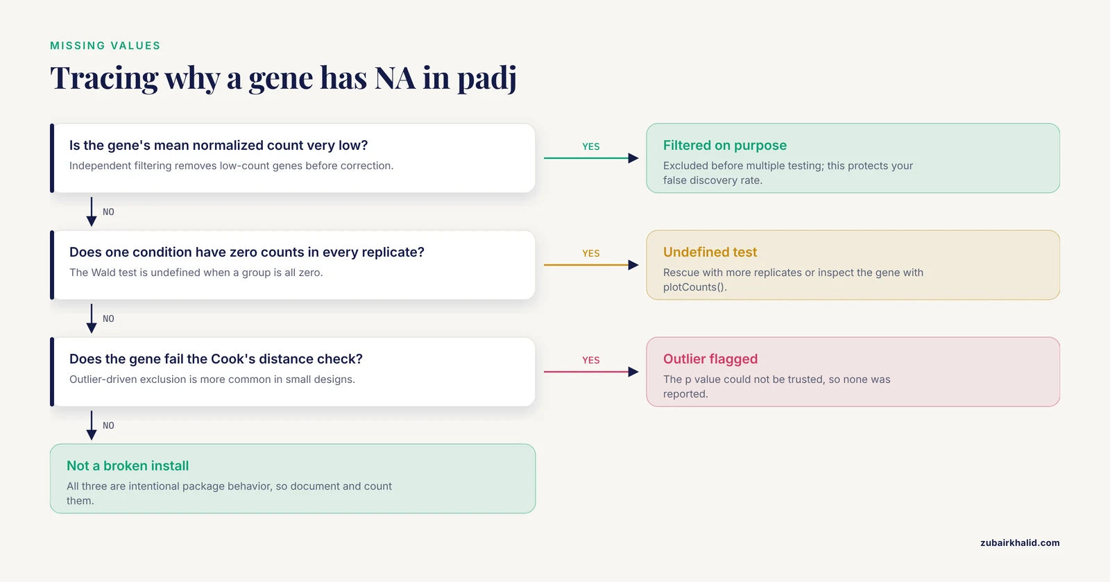
Three mechanisms produce NA adjusted p values, and each has a different remedy.

• Independent filtering. Genes with very low mean counts were excluded before correction. This is intentional behavior, not an error, and it protects your false discovery rate.
• All-zero or near-degenerate counts. If every replicate in one condition has zero counts for a gene, the Wald test is undefined. These genes can sometimes be rescued with more replicates or examined manually with plotCounts().
• Outlier-driven exclusion. Genes whose counts fail the Cook's distance checks, particularly in designs with small sample sizes, may be reported without a testable p value.

NA values in padj are one of the most frequently asked questions in DESeq2 results explained threads, and the answer is almost always one of these three mechanisms rather than a broken installation.

Diagnostics to Run Before You Trust Any Row

Interpretation should be preceded by a short battery of checks. Each takes minutes and prevents hours of downstream confusion.

• Size factors. Print sizeFactors(dds). Factors spread more than roughly 1.5-fold apart across conditions, especially if the spread aligns with your biological condition rather than with library preparation batches, warrant a hard look for composition biases.
• Dispersion plot. Run plotDispEsts(dds). The shrunken dispersion estimates should sit mostly on or below the fitted trend. Estimates sitting far above the trend across the board suggest the mean-variance model is a poor fit for your data.
• PCA. Apply vst() or rlog() transformation and run plotPCA(). Samples should separate by the biology you care about. Separation by date, lane, or operator instead signals batch structure that belongs in your design formula.
• p value histogram. As described above, check the shape of the raw p values.
• MA plot. plotMA(res) shows fold change against mean expression. Extreme fold changes at low baseMean values are a signature of unshrunken estimates, and comparing the MA plot before and after lfcShrink() makes the value of shrinkage immediately visible.
• Individual genes. Use plotCounts(dds, gene=..., intgroup="condition") on your top hits. A ranked list means little until you have looked at actual count distributions for a handful of genes, including a few you expect to change and a few you expect not to.

These checks are standard practice across DESeq2, edgeR, and related workflows, and the edgeR v4 documentation emphasizes analogous quality steps, including its improved statistical treatment for small counts that affects how low-count genes behave in the results [9].

How the Design Formula Shapes the Table

The design formula you passed to DESeq() determines what every number in the results table means. A few principles keep the interpretation honest.

• Include known nuisance factors. If samples were processed in two batches, use ~ batch + condition. Omitting a batch variable that is correlated with condition will inflate false positives for any gene whose counts track the batch.
• Order matters for interpretation only. In ~ batch + condition, the condition coefficient is adjusted for batch. The formula ~ condition + batch fits an identical model but changes which coefficient names resultsNames() reports by default.
• Interactions change the meaning of coefficients. With ~ genotype + treatment + genotype:treatment, the main effect coefficients describe effects within the reference genotype, not overall averages. Interpreting a main effect as a universal effect in an interaction design is a classic error.
• Use the likelihood ratio test for complex designs. When your question is whether a gene responds across a factor with more than two levels, or whether adding a term improves the model, the LRT compares the full and reduced designs and the results table reflects that comparison.

Paired and repeated-measures structures, donor effects, and time courses all follow from the same logic: every column in the results table is conditional on the model you specified, so interpretation of the table is inseparable from the design.

A Worked Filtering and Ranking Pass

Here is a compact, realistic sequence from fitted model to interpretable shortlist, using R syntax consistent with the DESeq2 package and the Bioconductor ecosystem.

res <- results(dds, contrast = c("condition", "treated", "control"), alpha = 0.05)
res_shrunk <- lfcShrink(dds, coef = "condition_treated_vs_control", type = "ashr")
sig <- subset(res, padj < 0.05 & !is.na(padj))
sig_ranked <- sig[order(sig$stat, decreasing = TRUE), ]
strong <- subset(sig, abs(log2FoldChange) >= 1 & baseMean >= 50)

Each line embodies one interpretation decision. The first fixes alpha at 0.05 and defines the contrast explicitly. The second produces shrunk effect sizes for ranking and plotting. The third applies the false discovery rate criterion. The fourth ranks by the Wald statistic, which balances effect size against uncertainty rather than by fold change alone, a practice that avoids promoting noisy low-count genes. The fifth adds minimal effect size and abundance floors to build a shortlist suitable for validation and enrichment.

What comes next depends on the question. For pathway-level interpretation, over-representation analysis and gene set enrichment analysis (GSEA) both consume the ranked or thresholded list. The corneal wound healing study cited above moved its filtered DEG list into GSEA, PANTHER, and Reactome enrichment and Cytoscape network analysis to arrive at mechanism-level conclusions about epithelial-to-mesenchymal transition and TGF beta signaling [8]. In a dengue severity study, DESeq2-normalized data and a 55-gene DEG list became the input features for machine learning classifiers distinguishing severe dengue from dengue fever, with transformer and convolutional architectures evaluated by ROC area under the curve [10]. Both workflows illustrate the same principle: the results table is an input to interpretation, never the endpoint.

Machine learning on DEG lists deserves one caution. If you select features on all samples and then evaluate the classifier on the same samples, performance estimates are optimistic. Split by sample before any feature selection step.

DESeq2 in Context: Alternatives and Complements

Knowing when to reach for something other than DESeq2 is part of competent interpretation.

edgeR. The other dominant negative binomial package in R for bioinformatics is edgeR, now at version 4, which pioneered empirical Bayes moderation for count data and supports quasi-likelihood inference, testing relative to a fold-change threshold, fractional counts, and pathway methods [9]. Results from edgeR and DESeq2 frequently overlap substantially on well-powered designs, and disagreements tend to concentrate on low-count genes, exactly where normalization and shrinkage choices matter most.

Formal benchmarks. A simulation study comparing eight differential methods, including edgeR, DESeq, DESeq2, baySeq, EBSeq, NOISeq, SAMSeq, and voom, found no significant differences in false discovery rate control, power, or stability across methods overall, but noted that EBSeq performed best with three samples per group while DESeq2 performed strongest as sample sizes increased to six or twelve per group [1]. The practical takeaway is that with three replicates per group, your fold changes and p values carry wide uncertainty regardless of method, and any single-gene conclusion from such a design should be framed accordingly.

Clustering-based alternatives. Methods such as MBCdeg3, which combine clustering with differential testing, have been benchmarked against edgeR, DESeq2, and TCC across simulation scenarios and offer an alternative route to identifying and classifying DEGs [11]. Their results will not match DESeq2 row for row, which is itself informative: when two defensible methods disagree about a gene, the honest interpretation is uncertainty, not a verdict.

Automated and graphical front ends. For teams without dedicated analysts, tools such as SeqExpressionAnalyser [6], RNA-SeqEZPZ [7], and GeneSEA Explorer [3] deliver DESeq2-style differential analyses with interactive visualization, and cloud-based protocols have demonstrated the full pipeline including pyDESeq2 differential analysis on free computing platforms [2]. Convenience does not change the statistics, so everything in this article applies to those outputs.

Single-cell data. DESeq2 results tables should not be interpreted from raw single-cell counts cell by cell. Single-cell differential methods battle high false positive rates, and approaches such as RankCompV3, which tests relative expression orderings of gene pairs, were developed specifically to control false positives and detect weak signals in scRNA-seq profiles [12]. Pseudobulking cells by sample and condition before differential testing, whether with DESeq2 or edgeR, remains the most robust default for multi-sample single-cell experiments.

What DESeq2 Cannot See

DESeq2 models differences in mean expression between conditions. Several biologically real patterns fall outside that frame, and a careful analyst knows the boundaries.

Non-monotonic expression profiles. Standard differential frameworks are optimized to detect monotonic mean shifts, where expression is consistently higher in one group. Patterns where a disease association appears at both low and high expression levels, sometimes called improper expression profiles, can be missed by conventional tests. Recent work evaluated generalized area under the ROC curve and length of the ROC curve indices as complementary screening tools for such profiles in RNA-seq data, using simulated negative binomial counts and a colorectal cancer microRNA dataset [13]. If your hypothesis involves heterogeneity within conditions rather than a between-group shift, plan a complementary analysis.

Variance and skewness. Two groups can share a nearly identical mean while differing sharply in variability or distribution shape. SIEVEseq addresses this with a compositional data framework that tests differential mean, variability, and skewness simultaneously, and its analysis of the Mayo RNA-seq Alzheimer dataset found that gene sets differing in all three moments predicted disease state better than mean differences alone, with functional enrichment revealing disease-related biology that DEG-only analysis missed [14]. The lesson for interpretation is that a gene absent from your DESeq2 list is not necessarily absent from the biology.

Cell-type composition. Bulk RNA-seq averages signals across mixed cell populations, so a fold change in bulk tissue can reflect a changing proportion of cell types rather than a per-cell expression change. A comparison of bulk and matched single-cell bronchoalveolar lavage data in equine asthma found that deconvolution primarily captured mRNA-derived cell proportions rather than true cell counts, with agreement with single-cell counts improving from a correlation of 0.62 to 0.83 after mRNA content correction [15]. When your bulk result could be a compositional effect, deconvolution or a matched single-cell comparison is the discriminating test.

Normalization sensitivity. The DEG list itself is sensitive to normalization choices, a variability that motivated tools aggregating differential results across multiple normalization methods using Shannon entropy [3] and prompted proposals such as gene-specific exponent-corrected normalization to remove residual library size effects [5]. Genes sitting at the edge of your significance threshold deserve skepticism precisely because small methodological changes can move them across it.

Common Mistakes and Limitations

• Filtering on raw p values. Reporting genes with pvalue < 0.05 instead of padj < 0.05 guarantees an inflated false discovery rate across thousands of tests. Use padj for all decisions you intend to defend.
• Reading the fold change without the contrast. Sign errors from ambiguous contrast direction are among the most common errors in DESeq2 results interpretation. Always record the numerator and denominator conditions alongside the table.
• Interpreting unshrunken fold changes at low counts. Genes with baseMean below roughly 20 can carry dramatic, unshrunken fold changes that shrink dramatically under lfcShrink(). Rank with shrunk estimates and check plotMA() before and after.
• Using TPM or FPKM as input. DESeq2 requires raw integer counts because the negative binomial model operates on count variance. TPM values destroy the count scale. Transcript-level estimates should be summarized to gene level with tximport-style tools [4].
• Treating padj as a posterior probability. The adjusted p value bounds the expected false discovery fraction among genes called at that threshold. It is not the probability that the gene is truly differential, and 0.049 versus 0.051 is not a meaningful boundary for individual genes.
• Ignoring NA padj values. Genes filtered by independent testing or flagged for outliers are not quietly insignificant. Document them and count them when you report how many genes were tested.
• Over-interpreting three-replicate designs. Benchmarks show that at three samples per group, method choice matters less than sample size, with EBSeq favored at that size and DESeq2 gaining its strongest performance at six or more samples per group [1]. Wide confidence intervals on fold changes are the honest description of such data.
• Forgetting composition effects. In heterogeneous tissues, fold changes may reflect cell-type proportions rather than per-cell regulation, and deconvolution comparisons show how easily the two are conflated [15].
• Assuming the DEG list is the whole story. Mean-shift testing misses non-monotonic profiles [13] and distributional changes in variance or skewness [14]. Genes with unchanged means can still carry strong disease-relevant signals.
• Cherry-picking thresholds after seeing the results. Choosing a fold change cutoff because it produces a convenient number of genes is circular. Predefine padj and effect size thresholds, or use lfcThreshold inside the test, before looking at the table.
• Skipping diagnostics. A results table computed on data with swapped samples, hidden batches, or a failed dispersion fit will still print tidy numbers. Run the size factor, PCA, dispersion, and p value histogram checks every time.
• Applying bulk rules to single-cell data. Cell-level DESeq2 calls on sparse single-cell counts are unreliable, and methods purpose-built for that setting control false positives better [12]. Pseudobulk by sample instead.

One honest limitation applies to every claim in this article. Statistical interpretation narrows uncertainty about population-level patterns in your dataset, and it cannot establish mechanism in a biological system without follow-up experiments.

Quick Review

• The six columns are baseMean, log2FoldChange, lfcSE, stat, pvalue, and padj, and mcols(res)$description documents each one inside your own results object.
• padj is the Benjamini-Hochberg adjusted p value and the primary calling criterion, and it bounds the expected false discovery fraction, not the probability that a gene is real.
• The direction of log2FoldChange follows from your contrast, and shrunk estimates from lfcShrink() are preferred for ranking and reporting effect sizes.
• NA values in padj come from independent filtering, undefined tests on all-zero groups, or outlier flags, and each has a distinct meaning.
• Run diagnostics before interpretation: size factor spread, plotDispEsts(), PCA on variance-stabilized counts, a p value histogram, an MA plot, and plotCounts() on candidate genes.
• DESeq2 tests mean shifts. Non-monotonic profiles, changes in variance or skewness, and cell-composition effects require complementary methods [13], [14], [15].
• With three replicates per group, fold change uncertainty is large under any method, and DESeq2 shows its strongest benchmark performance at six or more samples per group [1].

Frequently Asked Questions

What does the padj column in DESeq2 results mean?

It is the Benjamini-Hochberg adjusted p value, which estimates the smallest false discovery rate at which that gene would be called significant. Call genes using padj, typically below 0.05 or 0.10, because across thousands of tested genes the raw p value alone would flag large numbers of false positives.

Why do some genes have NA in the padj column?

Three causes cover nearly all cases: independent filtering removed low-count genes before multiple testing correction, the gene had zero counts in every sample of one group so the test was undefined, or the gene was flagged by the Cook's distance outlier procedure. These are intentional behaviors of the package, not installation problems.

Should I use the raw log2FoldChange or a shrunk estimate?

Use a shrunk estimate from lfcShrink(), for example with the apeglm or ashr types, for ranking, visualization, and reporting effect sizes, because shrinkage stabilizes noisy estimates from low-count genes. Keep the unshrunken estimates as the reproducible reference values, since they are what the Wald test and p values are based on.

Can I use TPM or FPKM values as input to DESeq2?

No. DESeq2 models raw integer counts with a negative binomial distribution and needs the count scale, including library size information, to estimate dispersion and fold changes correctly. Transcript-level abundance estimates from quantifiers should be summarized to gene-level estimated counts with tximport-style tools before differential analysis.

How many replicates do I need for trustworthy DESeq2 results?

Benchmarks indicate that DESeq2 delivers its strongest false discovery rate control, power, and stability at six or more samples per group, while at three samples per group alternatives such as EBSeq performed better and all methods carry substantial uncertainty. Whatever your design, report fold change standard errors alongside the fold changes so readers can judge the precision.

My gene has a small p value but a tiny fold change. Is it a real hit?

It is statistically real in the sense that the evidence rules out a zero effect, but a tiny fold change may not matter biologically. Decide effect size thresholds before analysis, or specify them inside the test with the lfcThreshold argument of results(), and remember that genes near the significance boundary can move across it with reasonable changes in normalization method.

Sources

1. An evaluation of RNA-seq differential analysis methods.
2. Streamline Protocol for Bulk-RNA Sequencing: From Data Extraction to Expression Analysis.
3. GeneSEA Explorer: An R Shiny Tool for Differential Gene Expression Analysis With Shannon's Entropy Aggregation.
4. Gene count estimation with pytximport enables reproducible analysis of bulk RNA sequencing data in Python.
5. Gene-specific exponent-corrected normalization for library size in bulk RNA-seq.
6. SeqExpressionAnalyser: An R Package for Automated End-to-End RNA-Seq Analysis From Reads to Differential Expression.
7. RNA-SeqEZPZ: A Point-and-Click Pipeline for Comprehensive Transcriptomics Analysis with Interactive Visualizations.
8. RNA-Seq Analysis Unraveling Novel Genes and Pathways Influencing Corneal Wound Healing.
9. edgeR v4: powerful differential analysis of sequencing data with expanded functionality and improved support for small counts and larger datasets.
10. Hybrid Feature Selection-Based Machine Learning and Deep Learning Framework for Biomarker Prediction From RNA-seq Data During Dengue Fever to Severe Dengue Progression.
11. Enhanced clustering-based differential expression analysis method for RNA-seq data.
12. RankCompV3: a differential expression analysis algorithm based on relative expression orderings and applications in single-cell RNA transcriptomics.
13. Complementary ROC-Derived Indices for Screening Improper Expression Profiles in RNA-Seq Differential Expression Analysis.
14. SIEVEseq: unified differential expression, variability, and skewness analyses using RNA-Seq data.
15. Cell-Type Deconvolution of Equine BALF RNA-Seq: A Critical Comparison with Matched Single-Cell Data.