How to Import Genomic Data into R: A Bioconductor Workflow
By Dr. Zubair Khalid, DVM, MS, PhD ·

By the end of this article you will be able to import genomic data into R using Bioconductor, the open-source software project that supplies most of the R ecosystem for bioinformatics. You will load raw sequencing reads from FASTQ files, alignments from BAM files, genomic intervals from BED and GTF files, coverage tracks from BigWig files, gene count matrices from transcript quantification tools, and chromatin interaction data from Hi-C or ChIA-PET experiments. You will also know how to check that each import worked, how to keep large datasets out of memory, and how to avoid the errors that come up most often in real projects.
What You Need Before You Start
Install these on your machine before typing any commands:
- R, version 4.4 or newer. Download it from CRAN.
- RStudio or any IDE you like. RStudio is convenient but not required.
- The
BiocManagerpackage, which installs and manages Bioconductor packages. Install it from CRAN withinstall.packages("BiocManager"). - Roughly 8 GB of RAM for the worked examples in this article. Whole-genome BAM files or single-cell matrices need more.
- Example data. For this walkthrough you can use any FASTQ, BAM, BED, GTF, and BigWig file you have. Public repositories such as the NCBI Sequence Read Archive and ENCODE host downloadable files for practice if your own data is not ready.
A note on versions. Bioconductor releases twice a year and each release is tied to a specific R version. If you upgrade R but not Bioconductor, or the other way around, packages will fail to install or behave unexpectedly. Run BiocManager::valid() after any upgrade to confirm the installation is consistent.
Why Bioconductor for Genomic Data
R for bioinformatics means R plus Bioconductor for most working analysts. The project provides three things that plain R does not.
First, purpose-built input and output. The ShortRead package, published in Bioinformatics, was designed specifically for input, quality assessment, and exploration of high-throughput sequencing data, and it connects those reads to the rest of the Bioconductor analysis environment [1]. Second, shared data containers. Classes such as GRanges, SummarizedExperiment, and GInteractions give every package the same vocabulary for genomic coordinates, per-feature measurements, and pairwise interactions. The InteractionSet package, for example, supplies the classes that represent genomic interactions from Hi-C and ChIA-PET experiments, and it deliberately builds on existing Bioconductor infrastructure so that higher-level packages remain interoperable [2]. Third, memory strategies. Assays keep getting bigger, and packages such as beachmat exist because single-cell experiments routinely produce matrices that no longer fit comfortably in RAM, requiring sparse or file-backed representations [3].
The payoff for learning one import layer is large. A well-formed Bioconductor object feeds directly into normalization, differential expression, visualization, and annotation packages without another format conversion. Published workflows across proteomics [4], CAGE and 5'-end data [5], and multi-state QTL analysis [6] all follow this same pattern: import once into a standard container, then analyze.
The Import Map: File Types, Packages, and Classes
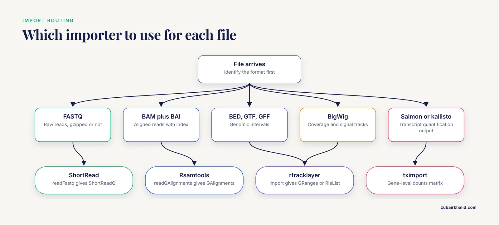
Use this table to route each file you receive to the right package and the object it produces.
| Data type | Common file format | Bioconductor package | Object you get |
|---|---|---|---|
| Raw reads | FASTQ, FASTQ.gz | ShortRead | ShortReadQ |
| Aligned reads | BAM, BAI index | Rsamtools, GenomicAlignments | GAlignments |
| Genomic intervals | BED, GTF, GFF | rtracklayer | GRanges |
| Coverage and signal tracks | BigWig, BedGraph | rtracklayer, tidyCoverage | GRanges, RleList |
| Transcript or gene quantification | Salmon, kallisto, featureCounts output | tximport | matrix or SummarizedExperiment |
| Count matrix with metadata | CSV, TSV, HDF5 | SummarizedExperiment, HDF5Array | SummarizedExperiment, DelayedMatrix |
| Chromatin interactions | BEDPE, Hi-C matrices | InteractionSet, GenomicInteractions | GInteractions, InteractionSet |
| Mass spectrometry | mzML, raw MS runs | MSnbase | OnDiskMSnExp |
| Pathway graphs | KGML, SBML, BioPAX | NetPathMiner | igraph-style networks |
| Public microbiome data | HMP 16S datasets | HMP16SData | SummarizedExperiment with taxonomy and tree |
The pattern to remember: every import ends in a Bioconductor class, not a plain data frame. That class carries coordinates, metadata, and assay values together, which is what makes downstream packages work without glue code.
Step 1: Install and Load the Packages
Open an R session and run:
install.packages("BiocManager")
BiocManager::install(c(
  "ShortRead", "Rsamtools", "GenomicAlignments",
  "rtracklayer", "tximport", "SummarizedExperiment",
  "GenomicRanges", "InteractionSet", "GenomicInteractions",
  "HDF5Array", "biomaRt"
))
BiocManager::valid()
The install step can take 10 to 30 minutes the first time because Bioconductor pulls in system libraries for compression, HDF5, and XML parsing. On Linux, install libcurl, libxml2, and libhdf5 development headers through your package manager first, or several installs will fail at the compile step.
Check the load:
library(ShortRead)
library(rtracklayer)
packageVersion("ShortRead")
#> [7] '1.62.0'
Your version number will differ by release. What matters is that no error appears and the version prints.
If you see Error in library(ShortRead) : there is no package called 'ShortRead', the package did not install. Rerun BiocManager::install("ShortRead") and read the full console output. The actual failure is usually several lines above the last message, often a missing system library or an R version below the release requirement.
Step 2: Import Raw Reads from FASTQ with ShortRead
FASTQ is where nearly every sequencing project begins. The ShortRead package handles input, quality assessment, and exploration of high-throughput sequence data and remains the standard entry point for reads in R [1].
A basic import of a gzipped FASTQ file:
library(ShortRead)

fq <- readFastq("sample_R1.fastq.gz")
fq
#> class: ShortReadQ
#> length: 25000000 reads; width: 150 cycles
The printed summary tells you the read count and read length immediately. Two quick checks confirm the file came in intact:
width(fq)          # vector of read lengths, should be uniform or nearly so
head(quality(fq))  # Phred-encoded quality strings
table(width(fq))   # a single value here means no variable-length contamination
For quality assessment over the whole file, ShortRead provides a report generator:
qa_summary <- qa("sample_R1.fastq.gz", type="fastq")
report(qa_summary, dest="qa_report", type="html")
This writes an HTML report covering read counts, base quality by cycle, and adapter content, the same read-level checks you would otherwise do with an external tool before aligning.
Now the tip that saves most beginners from their first crash. readFastq loads every read into memory. A 25 million read, 150 cycle file with qualities takes several gigabytes. For files at that scale or larger, stream in chunks with FastqStreamer:
streamer <- FastqStreamer("sample_R1.fastq.gz", n = 1e6)
total <- 0L
repeat {
  chunk <- yield(streamer)
  if (length(chunk) == 0) break
  total <- total + length(chunk)
}
total
#> [7] 25000000
close(streamer)
This loop reads one million reads at a time, so peak memory stays flat no matter how big the file is. Use yield counts to build your own filters, for example keeping reads above a length threshold and writing them back out with writeFastq.
Step 3: Import Alignments from BAM with Rsamtools and GenomicAlignments
Once reads are aligned, they live in BAM format with a .bai index alongside. The index is not optional. Random-access queries against a BAM file require it, and most import functions will refuse to run without one.
library(Rsamtools)
library(GenomicAlignments)

# Create the index if it does not exist
indexBam("sample.sorted.bam")

# Inspect the header before importing anything
scanBamHeader("sample.sorted.bam")$targets
#> chr1 chr2 chr3 ...
#> 248956422 242193529 198295559 ...
Read a whole chromosome into an alignments object:
param <- ScanBamParam(
  flag = scanBamFlag(isPaired = TRUE, isDuplicate = FALSE),
  what = c("qname", "flag", "mapq")
)
aln <- readGAlignments("sample.sorted.bam", param = param, use.names = TRUE)
aln
#> GAlignments object with 18234512 alignments and 2 metadata columns
Two parameters matter most. The flag argument filters at the C level, before anything reaches R, so filtering duplicates or unpaired reads here is far faster than filtering after import. The what argument limits which fields are read. Importing only qname, flag, and mapq is several times faster than importing every field when your analysis needs only a few columns.
For a genomic window rather than the whole chromosome, pass a GRanges in which. This is where the index pays off, because the reader seeks directly to the region instead of scanning the file:
which <- GRanges("chr1:1-1000000")
param <- ScanBamParam(which = which)
aln_region <- readGAlignments("sample.sorted.bam", param = param)
If you get Error: file has no index or a message about a missing .bai file, run indexBam() on the sorted BAM. If coordinates come back empty for a region you know has reads, check the sequence name style. The BAM header printed by scanBamHeader is the truth. If it says chr1 and you queried 1, the query silently returns nothing.
Step 4: Import Genomic Intervals from BED and GTF with rtracklayer
Gene models, peak calls, and variant regions usually arrive as BED, GTF, or GFF files. The rtracklayer package imports all of them into GRanges objects, the universal interval class in Bioconductor.
library(rtracklayer)
library(GenomicRanges)

peaks <- import("macs2_peaks.bed", format = "bed")
peaks
#> GRanges object with 45231 ranges and 2 metadata columns

genes <- import("gencode.gtf", format = "gtf")
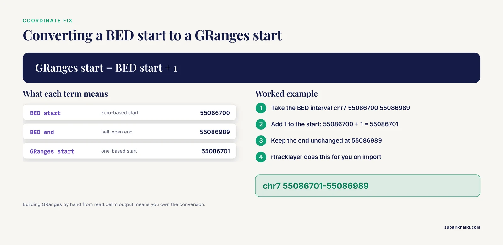
Understand the coordinate convention here, because it is the single most common silent bug in interval work. BED files use zero-based, half-open start coordinates. GRanges objects use one-based, closed coordinates. rtracklayer performs the conversion during import, so a BED interval recorded as chr7 55086700 55086989 arrives as chr7 55086701-55086989. If you ever read a BED file by hand with read.delim and build a GRanges yourself, you must add 1 to the start. Failing to do that shifts every interval by one base, which is invisible in summary output and quietly corrupts overlap counts.
Verify the import with standard accessors:
seqnames(peaks)        # which chromosomes are present
width(peaks)           # interval sizes
head(seqlevels(peaks)) # naming style, chr-prefixed or not
Check seqlevels against your BAM or annotation. If the peak file uses 1, 2, 3 and the alignment file uses chr1, chr2, chr3, later overlap operations will return zero results with no warning. Fix it before any comparison:
seqlevelsStyle(peaks) <- "UCSC" # adds the chr prefixThe seqlevelsStyle function guesses the style from a built-in database of known chromosome naming conventions, so it works for human, mouse, and most model organisms, but for a newly assembled genome you may need to set seqlevels() explicitly with a named mapping.
Step 5: Import BigWig Coverage Tracks
Coverage tracks from RNA-seq, ChIP-seq, or ATAC-seq pipelines usually ship as BigWig files. rtracklayer imports them, either whole-file or restricted to regions of interest:
# Whole chromosome coverage for one region
gr <- import("sample.coverage.bw",
             which = GRanges("chr1:1-1000000"))
gr
#> GRanges with a score column holding per-base coverage

# Whole-file import into run-length compressed form
cov <- import("sample.coverage.bw", as = "RleList")
cov$chr1
#> numeric-Rle of length 248956422 with N runs
The RleList representation is the memory-efficient one. It stores runs of identical values rather than one number per base, so a diploid human genome's coverage compresses to a manageable object as long as the track is not uniformly noisy.
For epigenomics work that centers on comparing many tracks over many features, the tidyCoverage package builds directly on SummarizedExperiment and provides CoverageExperiment and AggregatedCoverage classes for extracting coverage across thousands of loci and computing aggregated profiles, available for R 4.4 and Bioconductor 3.19 or newer [8]. That structure is the cleanest path when your question is aggregate-shaped, such as average signal over all enhancers in many samples.
The CAGEfightR package demonstrates how far a BigWig import layer can carry a full analysis. It imports data from BigWig files and uses them for fast, memory-efficient prediction and analysis of transcription start sites and enhancers, then hands the results to standard Bioconductor classes so differential expression tools such as limma, DESeq2, and edgeR apply directly [5]. The design lesson generalizes: import into standard classes, and every downstream tool works.
Step 6: Import Quantification Output with tximport
Most RNA-seq pipelines now use Salmon or kallisto to produce transcript-level abundance files rather than BAM files. The tximport package imports those outputs and summarizes them to the gene level, producing a count matrix ready for the standard differential expression packages.
library(tximport)

files <- c("sample1/quant.sf", "sample2/quant.sf", "sample3/quant.sf")
names(files) <- c("sample1", "sample2", "sample3")
tx2gene <- read.csv("tx2gene.csv")  # columns: TXNAME, GENEID

txi <- tximport(files, type = "salmon", tx2gene = tx2gene)
names(txi)
#> "abundance" "counts" "length" "countsFromAbundance"

head(txi$counts)
The countsFromAbundance argument controls how transcript-level abundance converts to gene-level counts. The default "no" works for most differential expression analyses with the standard downstream models. If your file paths are wrong, tximport stops immediately with Error: files do not exist, which is easy to fix. The subtle failure is a tx2gene table whose transcript identifiers do not match the quantification file, which produces missing rows rather than an error. Always check that nrow(txi$counts) matches the number of genes in your annotation and spot-check one gene's counts against the raw quant.sf file.
To wrap the counts with sample metadata in one object:
library(SummarizedExperiment)

coldata <- data.frame(
  condition = c("control", "treated", "treated"),
  row.names = c("sample1", "sample2", "sample3")
)
se <- SummarizedExperiment(
  assays = list(counts = txi$counts),
  colData = coldata
)
A SummarizedExperiment is the standard Bioconductor container for a feature-by-sample matrix plus feature metadata and sample metadata. Nearly every omics analysis package in the project accepts one as input, which is the practical reason to build it at import time rather than later.
Step 7: Import Chromatin Interaction Data
Chromosome conformation capture experiments produce pairwise genomic interactions rather than per-base tracks. Two Bioconductor packages define the infrastructure. InteractionSet provides the classes that represent genomic interactions and their associated experimental data, designed to exploit existing Bioconductor infrastructure and to be reused by higher-level packages [2]. GenomicInteractions builds on that foundation for processing, annotating, and visualizing data from Hi-C and ChIA-PET experiments [7].
A common text export from interaction callers is BEDPE, a tab-delimited format with the two anchor coordinates per line. There is no universal one-function importer for all BEDPE dialects, so the robust route is to read the table and construct the object explicitly:
library(InteractionSet)

bedpe <- read.delim("loops.bedpe", header = FALSE)
anchors1 <- GRanges(bedpe$V1, IRanges(bedpe$V2 + 1, bedpe$V3))
anchors2 <- GRanges(bedpe$V4, IRanges(bedpe$V5 + 1, bedpe$V6))

gi <- GInteractions(anchors1, anchors2)
gi$score <- bedpe$V7
gi
#> GInteractions object with 18400 interactions and 1 metadata column
Note the + 1 on the start coordinates. BEDPE follows the BED convention of zero-based starts, and constructing GRanges by hand means you own the conversion. Once interactions live in a GInteractions object, you can annotate them against promoters, count overlaps with feature sets, and pass them to the visualization methods in GenomicInteractions that were developed specifically for interaction datasets [7].
Step 8: Handle Data Too Large for Memory
Modern assays routinely produce matrices that exceed available RAM. Single-cell RNA-seq is the classic case, with expression values for every gene in every cell, and the field responded with sparse and file-backed matrix representations rather than dense in-memory ones [3].
The HDF5Array package stores a matrix on disk and reads blocks on demand through the DelayedArray interface:
library(HDF5Array)

big_counts <- read.csv("cell_counts.csv", row.names = 1)
h5 <- writeHDF5Array(as.matrix(big_counts), filepath = "counts.h5",
                     name = "counts")
h5
#> <20000 x 50000> HDF5Matrix object of type "double":
#>             [,1]      [,2] ...
The matrix now lives in counts.h5 on disk. Any code that indexes it, such as h5[1:100, 1:100], triggers a block read and returns a normal matrix slice. Column-wise operations on a single-cell matrix work without ever materializing the full object.
The memory and speed trade-off here is a genuine design decision, not an afterthought. beachmat was built to give C++ code in analysis packages uniform access across dense, sparse, and file-backed representations, and its evaluation quantified the clear memory and speed trade-off that motivates choosing a representation for a given dataset [3]. As a practical rule for analysts: use dense matrices under a few gigabytes, sparse matrices when most entries are zero, as they always are in single-cell count data, and HDF5-backed arrays when even the sparse form exceeds RAM or when you need the same matrix across multiple R sessions.
Step 9: Specialized Import Paths
Several data domains have their own import layers worth knowing about, because they compress what would otherwise be a multi-hour plumbing task into one call.
For proteomics, a published F1000Research workflow walks through mass spectrometry-based expression proteomics end to end, with an explicit early stage covering data import, pre-processing, and quality control separately for tandem mass tag and label-free quantitation datasets [4]. The MSnbase package supports that stage with an on-disk infrastructure that lets you handle large raw mass spectrometry experiments on commodity hardware, which is what makes full raw-file analysis feasible without a high-memory workstation [9].
For methylation arrays, preprocessing begins with raw signal intensities. The standard beta value for a CpG site is calculated as beta equals M divided by M plus U plus 100, where M and U are methylated and unmethylated signal intensities, and work on Illumina 450K data showed that quantile normalization of these intensities improves on the default GenomeStudio behavior [10]. The import lesson carries over: keep methylated and unmethylated channels separate at import and derive summaries later, because preprocessing choices act on the raw intensities, not on the derived betas.
For SNP arrays, the preprocessing literature makes the same point from the genotype side. Converting raw intensity measurements into usable genotype calls requires preprocessing steps that measurably affect measurement quality, and statistical methods applied during preprocessing improve accuracy relative to the manufacturer's ad hoc procedures [11]. Import raw intensities, not vendor calls, whenever the downstream analysis warrants it.
For public microbiome data, the HMP16SData approach demonstrates import by access rather than by file. It combines 16S taxonomic abundance data, public patient metadata, and phylogenetic trees as a single SummarizedExperiment-style data object, and provides an interface for approved dbGaP projects to retrieve and merge controlled-access metadata [12]. When a Bioconductor package exposes a public dataset directly, importing the file yourself is wasted effort.
For pathway data, NetPathMiner interfaces with KGML, SBML, and BioPAX input formats and represents the imported networks in metabolic, reaction, and gene forms [13]. For transcription factor motifs, TFBSTools handles profile matrices and can query the JASPAR database directly from R [14]. And for CAGE data, CAGEr provides collections of transcription start sites derived from most published CAGE datasets plus direct access to the FANTOM5 resource for numerous human and mouse cell and tissue types from within R [15], a reminder that the fastest import is often a packaged data resource rather than a downloaded file.
The tidyomics ecosystem is worth a mention for analysts who prefer tidyverse-style pipes. It bridges Bioconductor data frameworks to the tidy R paradigm and demonstrated its approach on 7.5 million peripheral blood mononuclear cells from the Human Cell Atlas spanning six data frameworks [16]. Import still produces Bioconductor classes. tidyomics changes how you manipulate them afterward, not how they arrive.
Checking That Your Import Worked
Every import deserves a validation step before analysis. A short checklist covers most cases:
- Dimensions. Print the object. Read count, gene count, or interval count should match what the upstream pipeline reported.
- Coordinates. For interval data, confirm chromosome naming style and that
width()values are plausible. A BED import where every interval is one base too short or too long signals a coordinate convention error. - Ranges. For alignments,
seqnames(table(seqnames(aln)))per chromosome should roughly match the composition you expect from the library type. - Metadata. For count matrices, verify
colnamesmatch your sample sheet exactly, including order, before any differential expression step. - One known value. Pick a single gene, peak, or CpG you have inspected in IGV or the source file and confirm its value in the imported object. One spot check catches more silent failures than any summary statistic.
Common Mistakes and Limitations
These are the failures that appear repeatedly in real projects, with their fixes.
Mixing coordinate systems. BED starts are zero-based, GRanges starts are one-based. When rtracklayer imports a BED file it converts for you. When you construct intervals manually from text files, you must convert. A one-base offset survives every sanity check that only looks at counts and destroys every overlap-based result.
Ignoring sequence name styles. 1 versus chr1 produces empty results, not errors. Always print seqlevels() from both objects you intend to compare and reconcile them before intersecting.
Loading whole files when streaming is available. readFastq on a 50 GB FASTQ file will exhaust memory and kill the R session with no useful traceback. FastqStreamer handles any file size at constant memory.
Working with an unindexed BAM. Region queries require the .bai index. Missing indexes produce hard errors from Rsamtools, and indexes built against an unsorted BAM produce wrong results silently. Sort first, index second.
Importing filtered or processed data when raw is needed. For methylation arrays, beta values computed by vendor software embed preprocessing decisions that later methods may want to change [10]. For SNP arrays, vendor genotype calls embed the manufacturer's calling procedure [11]. Import at the earliest stage your analysis might need, usually raw intensities.
Keeping everything in memory by default. A dense matrix that fits today may not fit the next experiment. Sparse and file-backed representations exist because high-throughput assays outgrew dense matrices, and the performance cost of block access is modest relative to the alternative of not running the analysis [3].
Skipping the version check after an R upgrade. A mismatched R and Bioconductor pair causes install failures with misleading messages. BiocManager::valid() diagnoses it in seconds.
Assuming import is quality control. A successful import proves the file parsed. It says nothing about read quality, mapping rate, batch effects, or sample swaps. Run package-native QA after import, such as the ShortRead report for reads [1], and the QC stages in the published proteomics workflow before differential analysis [4].
Discarding metadata at the boundary. Sample annotations lost during import must be reconstructed later, often imperfectly. Carry colData, condition labels, and batch information into the container at import time.
Tips for Reliable Bioconductor Imports
- Write the import as a script, never interactively only. A script that starts from raw files and ends at a saved
RDataorRDSobject is reproducible. A session history is not. - Save intermediate objects in native R format with
saveRDS(). RDS preserves Bioconductor classes exactly, unlike CSV round-trips which flattenGRangesobjects and lose metadata structure. - Fix chromosome styles in one central script at import time. Every downstream script inherits clean, matching seqlevels.
- Import only the columns and regions you need.
ScanBamParam(what = ...)and thewhichargument cut BAM import time by large factors on chromosome-scale data. - Record package versions in the output.
sessionInfo()at the end of every script costs nothing and makes results traceable to exact software versions when a reviewer or collaborator asks. - Prefer packaged data resources over manual downloads when they exist. Direct access to resources such as FANTOM5 transcription start sites through CAGEr [15] or Human Microbiome Project data through HMP16SData [12] removes download, parsing, and identifier-matching errors from your workflow.
Frequently Asked Questions
What does it mean to import genomic data into R?
It means reading files such as FASTQ, BAM, BED, GTF, BigWig, or count matrices into Bioconductor data classes so that genomic coordinates, measurements, and metadata stay linked together. Packages like ShortRead, rtracklayer, and tximport perform these conversions and produce objects that the rest of the Bioconductor ecosystem accepts directly [1].
Which Bioconductor package should I use for FASTQ files?
ShortRead. It was designed for input, quality assessment, and exploration of high-throughput sequencing data, and its readFastq function imports FASTQ into a ShortReadQ object while FastqStreamer streams large files in fixed-size chunks to keep memory flat [1].
How do I import a BAM file into R?
Use Rsamtools with GenomicAlignments. Index the BAM with indexBam(), restrict fields and flags with ScanBamParam(), then call readGAlignments() to get alignments in a GAlignments object. Always sort and index the BAM before importing, and filter with the flag argument so unwanted reads never reach R.
How do I import BigWig coverage files into R?
Use rtracklayer. import("file.bw", which = myGRanges) returns coverage for selected regions as a GRanges, and passing as = "RleList" returns run-length compressed coverage for efficient whole-genome storage. Packages such as CAGEfightR build entire analyses on top of BigWig imports [5].
How do I handle a count matrix that is too big for memory?
Store it on disk with HDF5Array and access it through the DelayedArray interface, which reads blocks on demand. Sparse matrices help when most values are zero, as in single-cell data. The beachmat project defined the memory and speed trade-off between these representations for exactly this problem [3].
What are the most common mistakes when importing genomic data into R?
Mixing zero-based BED coordinates with one-based GRanges coordinates, mismatching chr1 versus 1 sequence names, importing from unindexed or unsorted BAM files, loading whole files into memory instead of streaming, and treating a successful import as proof of data quality. Each has a one-line fix covered in the mistakes section above.
Do I need to know the command line to import genomic data into R?
No. Bioconductor handles reading, decompression, and parsing from within R for FASTQ, BAM, BED, GTF, BigWig, HDF5, and mass spectrometry formats. Command-line tools are still useful for upstream steps such as alignment, but the import step itself is pure R.
Can Bioconductor import data from public repositories directly?
Yes, for many resources. HMP16SData retrieves Human Microbiome Project 16S data with taxonomy, metadata, and phylogenetic trees as a single data object [12], and CAGEr provides direct access to the FANTOM5 transcription start site resource for human and mouse from within R [15]. Where such a package exists, it is faster and less error-prone than downloading and parsing files manually.
Sources
- ShortRead: a bioconductor package for input, quality assessment and exploration of high-throughput sequence data.
- Infrastructure for genomic interactions: Bioconductor classes for Hi-C, ChIA-PET and related experiments.
- beachmat: A Bioconductor C++ API for accessing high-throughput biological data from a variety of R matrix types.
- A Bioconductor workflow for processing, evaluating, and interpreting expression proteomics data.
- CAGEfightR: analysis of 5'-end data using R/Bioconductor.
- Orchestrating multi-state QTL analysis with Bioconductor.
- GenomicInteractions: An R/Bioconductor package for manipulating and investigating chromatin interaction data.
- Epigenomics coverage data extraction and aggregation in R with tidyCoverage.
- MSnbase, Efficient and Elegant R-Based Processing and Visualization of Raw Mass Spectrometry Data.
- A data-driven approach to preprocessing Illumina 450K methylation array data.
- Exploration, normalization, and genotype calls of high-density oligonucleotide SNP array data.
- Invited Commentary: Improving the Accessibility of Human Microbiome Project Data Through Integration With R/Bioconductor.
- NetPathMiner: R/Bioconductor package for network path mining through gene expression.
- TFBSTools: an R/bioconductor package for transcription factor binding site analysis.
- CAGEr: precise TSS data retrieval and high-resolution promoterome mining for integrative analyses.
- The tidyomics ecosystem: enhancing omic data analyses.