ggplot2 Genomic Data Errors: Causes and Fixes
By Dr. Zubair Khalid, DVM, MS, PhD ·

ggplot2 is the default plotting layer in r for bioinformatics, and most genomic plotting failures trace back to a handful of root causes rather than to ggplot2 itself. The single most common cause is this: the data frame you think you are passing to ggplot() is not the data frame ggplot2 is actually seeing, or one of its columns has the wrong type. A chromosome column stored as text ("chr1", "chr2") gets mapped to a continuous axis and throws Error: Discrete value supplied to continuous scale. A wide genotype matrix with one column per sample gets passed to aes() as if it were long-format data, and every geom fails at once.
The first thing to check, before anything else, is the actual structure of the object immediately before the plotting call. Run dplyr::glimpse(plot_df) or str(plot_df) on the exact data frame you are handing to ggplot(), not on an earlier version of it. Nine out of ten ggplot2 genomic data errors become obvious in that output. This article walks through the causes of ggplot2 genomic data errors from most common to rarest, explains the mechanism behind each failure, gives a diagnostic sequence you can follow in under five minutes, and closes with prevention practices that keep genomic figures reproducible.
Why Genomic Data Breaks ggplot2 Differently
Genomic workflows produce data shapes that general ggplot2 tutorials rarely cover. Variant call format (VCF) files are semi-structured text with per-sample genotype columns buried in INFO and FORMAT fields. Genome browser style figures need per-chromosome coordinate tracks. Linkage disequilibrium (LD) analyses produce pairwise matrices that must be melted before they can be drawn as heatmaps. Population genetic summaries produce one statistic per population per locus, which is naturally long data, while the raw genotypes behind them are naturally wide.
This mismatch between data shape and plotting shape is why published genomic visualization tools keep reinventing the same wrappers. The yEvo Mutation Browser, an R Shiny tool for visualizing mutations in evolved yeast lines, provides an interactive chromosome map, mutation type summaries, and a gene level viewer precisely because building these views from scratch with raw plotting calls is hard for most users [1]. XVCF wraps vcfR and maftools behind a graphical interface to summarize read depth, mapping quality, genotype, and allele frequency from VCF files without requiring users to write the underlying plotting code themselves [2]. LDblockR was built as a single R native object model linking heterogeneous genotype inputs to LD statistics and publication ready visualization, explicitly because the usual workflow requires format conversion between VCF, HapMap, PLINK BED, and numeric genotype matrices before any plotting can happen [3]. And the thyroid cancer precision oncology literature describes standard pipelines that lean on ggplot2 together with dplyr, ggrepel, and tidyr to map mutations from TCGA and cBioPortal data [4].
The lesson from all of these tools is consistent: the errors are predictable, they come from data structure and data type mismatches, and they can be fixed at the source.
Troubleshooting Table
Use this table as your first reference. Work top to bottom, since the earlier rows cover the majority of real failures.
| Symptom | Likely cause | How to confirm | Fix |
|---|---|---|---|
Error: Discrete value supplied to continuous scale | A column ggplot2 expects to be numeric (position, read depth, p value) is a factor or character | str(plot_df) on the exact object passed to ggplot() | Convert with as.numeric(). If it has non-numeric suffixes, strip them with readr::parse_number() |
Error: Continuous value supplied to discrete scale | A numeric column mapped to aes(color = ) or aes(fill = ) where the scale expects categories | Check the mapped column with class() | Wrap the column in factor() if you want categories, or use a continuous gradient scale |
Warning: Removed N rows containing missing values | NA values in the mapped aesthetics | sum(is.na(plot_df$x)) | Decide deliberately: filter with tidyr::drop_na() or keep the points with geom_point(na.rm = TRUE) after you know why they are missing |
Error: object 'x' not found inside aes() | Column name typo, or the pipe dropped the data frame before ggplot() | Print the object one step before the plot | Fix the name, and confirm data is the first argument to ggplot() |
Aesthetics must be either length 1 or the same as the data | A hardcoded vector passed into aes() with the wrong length | length(your_vector) vs nrow(plot_df) | Move the vector into the data frame as a column and map it by name |
| Chromosomes plot as 1, 10, 11, 2 | Chromosome names are characters or unordered factors, so ggplot2 sorts them alphabetically | levels(factor(plot_df$chr)) | Refactor with explicit levels, for example factor(chr, levels = paste0("chr", 1:22)) |
Error: Insufficient values in manual scale | More factor levels than colors supplied to scale_fill_manual() | length(levels(plot_df$var)) | Add colors to the values argument or switch to scale_fill_viridis_d() |
position_dodge() requires non-overlapping x intervals | Dodging bar or box geoms where the x variable is continuous or the group aesthetic is missing | Inspect the discrete x variable | Set aes(group = ) explicitly or use geom_col(position = position_dodge(width = 0.9)) on a discrete x |
| Points silently vanish from a log-scale plot | Read depths or allele frequencies of exactly zero become -Inf on a log axis | min(plot_df$y, na.rm = TRUE) | Filter zeros with intent, or use scale_y_log10() with a small pseudocount, or scales::pseudo_log_trans() |
Error in ggplot(...) : could not find function "ggplot" | ggplot2 installed but not attached, or not installed | search() lists attached packages | library(ggplot2) or install.packages("ggplot2") |
| R session aborts or memory spikes when plotting a large VCF | The full genotype matrix plus reshaped long data all live in memory at once | object.size(genotype_matrix) | Plot a subset, rasterize, or move parsing to a leaner toolchain (see the memory section below) |
The Causes, From Most Common to Rarest
Cause 1: Untidy data, wide when it should be long
ggplot2 expects tidy data: one observation per row, one variable per column. Genomic data is almost never tidy by default. A genotype matrix from PLINK or from vcfR has one row per variant and one column per sample, which is the opposite of what aes(x = sample, y = genotype, fill = allele) needs. A per-gene expression table has genes as rows and conditions as columns. An LD matrix from LDblockR style analysis has one r² value per cell, which must be melted before any heatmap geom can read it [3].
The failure mode is usually silent at first. You map a wide column range to aes(x = pos, y = Sample1) and get one geom per sample, or you get an error because ggplot2 tried to interpret sample names as a variable. The fix is a reshape step in the pipeline:
library(tidyr)
geno_long <- geno_wide |>
  pivot_longer(cols = -c(CHROM, POS, REF, ALT),
               names_to = "sample",
               values_to = "gt")
The native pipe |> requires R 4.1 or later. On older versions, use magrittr's %>%. The two behave identically for this pattern. After reshaping, glimpse(geno_long) should show one row per sample per variant, and the ggplot call becomes straightforward. The thyroid cancer workflows that use ggplot2 with dplyr and tidyr for TCGA mutation data follow exactly this pattern, reshaping first and plotting second [4].
A related trap: stat_count() is the default stat for geom_bar(), and it counts rows. If your data already contains counts, for example a table of variant types with a frequency column, geom_bar() throws Error: stat_count() can only have an x or y aesthetic or double counts. Use geom_col() instead, which passes the values through with stat = "identity".
Cause 2: Type mismatches between columns and scales
Every aesthetic in ggplot2 has an expected data type. Continuous scales want numeric vectors. Discrete scales want factors or characters. Genomic data breaks this constantly because chromosome identifiers, gene names, and variant classifications look numeric at a glance but are not.
Chromosome names are the classic case. If chr is a plain character column, aes(x = chr) treats it as discrete, which is usually what you want, but the alphabetical ordering puts chr10 after chr1 and before chr2. If instead you stripped the "chr" prefix with as.numeric(), the X and Y chromosomes and any unplaced scaffolds become NA, and you get rows removed warnings. The robust pattern is an explicit factor:
chr_levels <- c(paste0(1:22), "X", "Y", "M")
plot_df$chr <- factor(plot_df$chr, levels = chr_levels)
The reverse case bites with allele frequency data. ploidyfrost, a reference free ploidy estimator, visualizes allele frequency distributions with ggplot2 and models them with a Gaussian mixture, because allele frequencies carry ploidy signal in where their peaks fall [5]. If a column of allele frequencies was read in as character (common when a VCF export includes formatting), mapping it to aes(x = af) produces Error: Discrete value supplied to continuous scale. Confirm with class(plot_df$af) and convert with as.numeric().
Quality metrics from VCF files have the same exposure. XVCF extracts read depth, mapping quality, genotype, and allele frequency from unannotated VCF data for quality control summaries [2]. Those fields arrive as text from many parsers, and every one of them needs an explicit numeric conversion before any continuous ggplot2 scale will accept it.
Cause 3: Missing values treated as a mystery instead of a decision
The warning Removed N rows containing missing values (geom_point()) is not an error. It is ggplot2 telling you that N rows had NA in a mapped aesthetic and were dropped from the drawing. In genomic work this is usually meaningful: variants with no genotype call, sites with depth zero, genes with no expression measurement. The error people make is silencing the warning before reading it.
The diagnostic is one line:
sum(is.na(plot_df$depth))Then make a deliberate choice. If the missing values are uninformative, filter them upstream with tidyr::drop_na(plot_df, depth) so the filtering is documented in your script. If the missing values are themselves the message (for example, missing genotypes clustering on one chromosome), keep them visible by plotting a missing indicator, or by using na.rm = TRUE on the geom to suppress the warning once you have confirmed the count. Rows that vanish silently on a log scale are the more dangerous variant of this problem, covered below.
Cause 4: Data loss through pipe and layer mechanics
The error object 'x' not found inside an aes() mapping has three usual mechanisms in genomic scripts.
First, a typo in the column name. R column names from VCF INFO fields often contain dots or underscores, and DP50 is not dp50.
Second, the data frame never reached ggplot(). This happens when the pipe chain computes something in the middle and the plot call inherits the wrong object:
# Broken: summarise() returns a summary table, not the per-variant data
df |> summarise(mean_dp = mean(depth)) |> ggplot(aes(x = depth))
Third, a layer receives different data than the base plot. ggplot2 allows per-layer data, and a common genomic pattern is a base genome track plus an overlay of hits from a separate hits data frame. If the overlay layer's data lacks the faceting variable used in facet_wrap(), you get Error: At least one layer must contain all faceting variables. The fix is to make sure every layer's data carries the faceting columns, usually by a dplyr::left_join() before plotting rather than by juggling two data frames inside one plot object.
A fourth variant of this family is the hardcoded aesthetic vector. Writing aes(color = c("red", "blue")) with a two element vector against a ten thousand row data frame throws Aesthetics must be either length 1 or the same as the data. Colors, labels, and line types belong in columns of the data frame, mapped by name. For labeled points in dense Manhattan style plots, use ggrepel, which is the standard companion to ggplot2 for non-overlapping text labels and appears in documented genomic pipelines for exactly this reason [4].
Cause 5: Coordinate and axis problems specific to genome data
Genomic coordinates introduce failure modes that general plotting data does not.
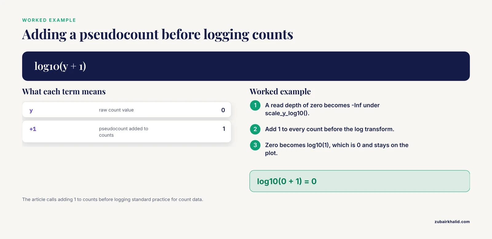
Log scales and zeros. Read depths, coverage, p values, and counts can be zero or negative. scale_y_log10() turns zero into -Inf and the points disappear without a hard error, sometimes with only a removed-rows warning. Confirm with min(plot_df$y, na.rm = TRUE). The fixes, in order of honesty: filter zeros with a documented reason, add a pseudocount (adding 1 to counts before logging is standard practice for count data), or use scale_y_continuous(trans = scales::pseudo_log_trans()) when the data spans negative and positive values. Allele frequency data plotted on a linear scale between 0 and 1 faces a related issue, and ploidyfrost's approach of visualizing the full allele frequency distribution with ggplot2 rather than plotting only summary values exists precisely because the shape of that distribution, including its tails, is the signal [5].
X axis ordering. Covered above under type mismatches, but worth restating as its own failure class because it does not error at all. The plot renders, looks correct, and quietly puts chromosome 10 between 1 and 2. Peer reviewers catch this more often than scripts do. Explicit factor levels fix it permanently.
Faceting per chromosome. facet_wrap(~ chr, scales = "free_x") is the right tool for per-chromosome coverage tracks, but it fails when the faceting variable is missing from any layer's data, and it produces unreadable output when chromosome names are unordered factors. Combine the factor-level fix with a single joined data frame and both problems disappear.
Cause 6: Scale and palette exhaustion
Error: Insufficient values in manual scale fires when you hardcode a palette shorter than the number of factor levels. Genomic data inflates level counts easily: a categorization of mutation types, a set of sample populations, a panel of resistance genes. The E. coli genomic surveillance literature covering over thirty thousand isolates across 126 countries illustrates how many categories resistance and typing analyses can accumulate, and such data is visualized with statistical and plotting tools in R and Python [6]. Hardcoding a named color vector for a panel that grows every update guarantees this error eventually.
Two robust solutions:
# Option 1: programmatic palette from a stable base
n_levels <- length(levels(plot_df$variant_class))
pal <- scales::hue_pal()(n_levels)

# Option 2: let a perceptually uniform scale size itself
scale_fill_viridis_d()
Cause 7: Memory pressure with large variant datasets
Large VCF files and genotype matrices break ggplot2 indirectly. ggplot2 copies and reshapes data at plot build time, so a wide matrix of millions of genotype calls, once pivoted long, can multiply memory use severalfold and abort the R session. The benchmark comparison behind SNPio, a Python native framework for population genomic data processing, is informative here: SNPio parsed and filtered VCF data faster than the R based comparators vcfR and SNPfiltR, but used more memory, because it retains genotype arrays, metadata, and provenance tracking attributes in memory [7]. The general lesson is that genotype-aware objects that hold everything in RAM trade memory for convenience, and any plotting layer on top of them inherits that cost.
Practical fixes, in order of preference:
- Plot a subset. Filter to the region, chromosome, or variant class you are actually visualizing before the reshape.
- Rasterize dense layers. Add
geom_point(alpha = 0.2, raster = TRUE)from ggrastr, or aggregate to binned counts withstat_bin()so the number of drawn shapes stays small. - Parse lean. If you only need the GT field, extract it and drop the rest of the VCF record early, rather than carrying full records through the plotting pipeline.
- Move heavy preprocessing out of the plotting layer. SNPio exists because fragmented preprocessing scripts between raw genotype files and downstream analysis introduce friction, and consolidating parsing and filtering upstream of visualization is the architectural fix [7].
The same principle appears at whole pipeline scale. CGAS, a chloroplast genomics pipeline, integrates R based visualizations only where graphical output is required inside an otherwise automated workflow, rather than building interactive plots over the full intermediate dataset [8].
Cause 8: Package versions, deprecations, and extension conflicts
ggplot2 deprecations produce warnings rather than errors, and they cluster in older analysis scripts. Since ggplot2 3.4.0, size is deprecated in favor of linewidth for line-like geoms such as geom_line(), geom_path(), and geom_errorbar(). Scripts written years ago still run but emit deprecation warnings, and a future release will turn these into failures. Update aes(size = ) on line geoms to aes(linewidth = ).
Extension package conflicts are the rarer but harder class. Genomic visualization in R often mixes ggplot2 with Bioconductor or CRAN extension objects: phylogenetic trees from ggtree, genomic tracks from ggbio, enrichment plots from clusterProfiler, and network views from mixOmics based multi-omics workflows [9]. These extensions wrap ggplot2 and add their own geom_ and stat_ functions. When two packages export functions with the same name, the one attached last masks the other. Confirm which version is running with conflicted::conflict_scientific() style checks or simply find("geom_text"). The fix is to be explicit with namespacing, for example ggplot2::geom_point(), in scripts that load many extension packages. The microbial multi-omics resource published in Microbial Genomics structures its analysis as a multi-step R Markdown workflow using mixOmics and clusterProfiler, and that document-driven structure is also the simplest defense against silent version drift, because every library call is recorded in the rendered output [9].
Cause 9: Malformed or mismatched input objects at the Bioconductor boundary
The rarest and most confusing errors happen when Bioconductor objects meet ggplot2. A GRanges object, a SummarizedExperiment, or a VCF read in through VariantAnnotation::readVcf() is not a data frame, and ggplot2's default fortify() method does not know what to do with it. You get Error: data must be a data frame, or other objects coercible by fortify(), not a S4 object or similar.
The fix is an explicit conversion step before plotting:
library(VariantAnnotation)
vcf <- readVcf("variants.vcf.gz")
vdf <- as.data.frame(rowRanges(vcf))
vdf$depth <- info(vcf)$DP
For a bioconductor tutorial style rule of thumb: convert S4 containers to plain data frames at a clearly marked point in the script, then let everything downstream of that point be standard tidyverse and ggplot2 code. Specialized packages such as ggbio handle the conversion internally for genomic tracks, but generic ggplot2 calls do not. Any reader following a bioconductor tutorial should watch for this boundary, because the tutorial's conversion step is often the line their own script is missing.
A Diagnostic Sequence That Works
When a ggplot2 genomic plot fails and the cause is not immediately visible, run this sequence in order. It resolves most failures in under five minutes.
- Print the data.
dplyr::glimpse(plot_df)immediately before the ggplot call. Confirm column names, types, and row count on the actual object being plotted. - Read the error bottom up. ggplot2 error traces list the innermost failing operation last. The line that names a geom or a stat is the one that failed, and the line above it usually names the aesthetic involved.
- Check types of mapped columns only. You do not need to fix the whole data frame, only the columns referenced inside
aes(). - Count missing values in mapped columns with
colSums(is.na(plot_df[, mapped_cols])). - Check factor levels for any discrete axis, especially chromosome, with
levels(). - If a plot renders but looks wrong, check ordering and counts:
table(plot_df$chr)reveals both alphabetical ordering artifacts and empty categories at a glance. - Reproduce on a subset.
plot_df |> slice_head(n = 500) |> ggplot(...). If the subset plots, the failure is data volume, not code, and the memory fixes above apply. - Check loaded packages and versions with
sessionInfo()when the error mentions a function that should exist.
Prevention Practices
Reshape once, plot many. Every genomic project benefits from a single documented tidy-data step: variants melted to long format, sample metadata joined by a stable sample ID, chromosome and position converted to typed columns. Every downstream figure then reads from the same clean object. This is the structural principle behind LDblockR's single object model linking genotype inputs to statistics and publication ready visualization [3], and behind the multi-step R Markdown structure of the microbial multi-omics workflow, where each transformation is recorded in rendered output [9].
Assert your expectations. A two-line check before plotting catches most silent failures:
stopifnot(is.numeric(plot_df$depth), is.factor(plot_df$chr))
stopifnot(!any(is.na(plot_df$depth)) || TRUE)
The second form documents that you know NAs exist and have decided to keep them.
Pin versions and record sessions. Save sessionInfo() output with every figure script. Educational and pipeline tools alike emphasize reproducibility: the yEvo browser exists partly to give students a stable, interpretable view of sequencing results they generated themselves [1], and CGAS delivers reproducible, scalable comparative genomics outputs as an explicit design goal [8]. A pinned renv.lock or a recorded sessionInfo() block in the script header serves the same purpose for your own figures.
Keep preprocessing and plotting separate. The friction between raw genotype files, quality control decisions, statistical analyses, and downstream visualization is a documented pain point in population genomics workflows [7]. Solving it architecturally, with a parsing and filtering stage that writes clean intermediate files, means ggplot2 errors stay in the plotting layer where they are cheap to diagnose, rather than cascading from parsing code three steps upstream.
Label deliberately. Dense genomic scatter plots need non-overlapping labels, and ggrepel is the standard tool for it in documented ggplot2 pipelines [4]. Default geom_text() on a Manhattan plot produces an unreadable smear, which is a real failure even though no error is thrown.
Common Mistakes and Limitations
These are the mistakes that show up repeatedly in real analysis sessions, stated so you can check your own scripts against them.
Silencing warnings during iteration. The removed-rows warning is diagnostic information about your variants. Suppressing it globally with na.rm = TRUE before checking sum(is.na()) turns a data quality problem into an invisible one. Check first, then suppress with a comment explaining the count.
Fixing types at the plot instead of at the source. Writing aes(x = as.numeric(af)) inside a ggplot call works, but it hides the conversion from the rest of the pipeline, and the same column will fail again in the next figure or in a model. Convert once, upstream, with validation.
Assuming alphabetical factor order is meaningful. It never is for chromosomes, bands, or gene panels. Every discrete axis in a genomic figure should have explicit levels, even when the current ordering happens to look right.
Plotting all data when the question concerns a region. Genome-wide default views overplot hundreds of thousands of points, exhaust palettes, and consume memory. Subset to the region of interest unless the genome-wide view is itself the point.
Mixing interactive and static plotting expectations. Tools built on R Shiny, such as XVCF for VCF quality control summaries [2] and the yEvo browser [1], add interactivity on top of static plotting logic. A figure that fails in static ggplot2 will fail the same way inside a Shiny render call, and the debugging sequence is identical. Fix the ggplot2 error first, then wrap it.
One limitation deserves a plain statement. These fixes cover plotting layer failures, and they will not rescue an analysis built on incorrectly parsed variant data. If depth, genotype, or coordinate fields were extracted wrong upstream, ggplot2 will faithfully draw the wrong numbers. Validate the parsing step against a few variants by hand before trusting any figure it produces.
Frequently Asked Questions
Why does ggplot2 say "Discrete value supplied to continuous scale" with my variant table?
A column you mapped to a continuous aesthetic is stored as a character or factor. This is most common for read depth, allele frequency, and position fields parsed from text-based formats. Run str() on the exact data frame passed to ggplot(), identify the mapped column with the wrong class, and convert it with as.numeric() upstream of the plot.
Why do points disappear from my log-scale read depth plot without an error?
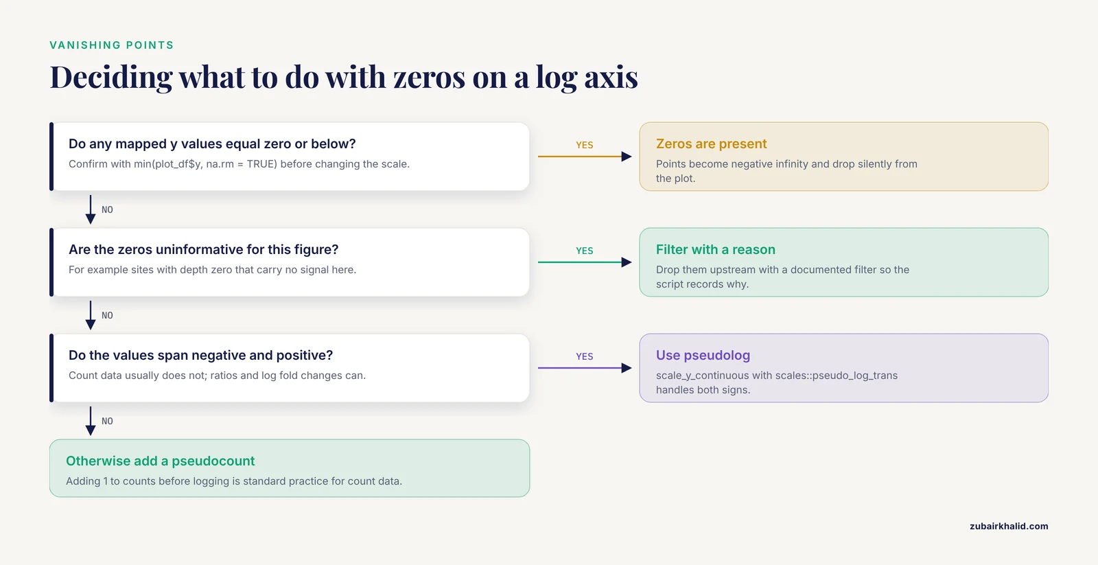
Values of zero or below become negative infinity on a log axis and are dropped. Check min() on the y variable to confirm, then either filter zeros with a documented reason, add a small pseudocount for count data, or switch to a pseudolog transformation.
How do I plot a VCF genotype matrix as a heatmap in ggplot2?
Melt the matrix to long format with pivot_longer() so each row is one sample by one variant, then use geom_tile(aes(x = sample, y = variant_id, fill = gt)). Genotype calls need to be numeric (for example 0, 1, 2 for dose) or a factor for a discrete fill scale. For large matrices, subset to a region first to avoid memory problems.
Why does my bar chart of variant types throw a stat_count error?
geom_bar() counts rows by default. If your table already contains a count or frequency column, use geom_col() instead, which draws the values as they are. Using geom_bar() on pre-counted data double counts or errors out.
Why do my chromosomes plot in the wrong order along the x axis?
Chromosome names stored as characters sort alphabetically, placing 10 between 1 and 2. Convert the chromosome column to a factor with explicit levels ordered by number, then by X, Y, and mitochondrial or unplaced contigs, before plotting.
R runs out of memory when I plot large variant datasets. What do I do?
Subset to the data the figure actually needs, aggregate dense layers into bins, and extract only the genotype or INFO fields you will plot rather than carrying full records. Genotype-aware tools that keep everything in memory trade RAM for convenience, so heavy parsing and filtering should happen upstream of the plotting layer, in a leaner step.
Should I use ggplot2, base graphics, or specialized Bioconductor tools for genomic tracks?
Use ggplot2 for most publication figures, and reach for specialized Bioconductor packages such as ggbio or ggtree when the figure needs genome tracks, gene models, or trees drawn from S4 objects. In either case, convert complex Bioconductor containers to plain data frames at one clearly marked point, which keeps debugging simple.
How do I make ggplot2 genomic figures reproducible across machines and collaborators?
Record the package versions with sessionInfo() or a lockfile, write every transformation from raw files to the plotted data frame in a single script, and keep parsing, reshaping, and plotting as separate stages. Document-driven workflows in R Markdown make this automatic, since the rendered output captures every library call and transformation.
Sources
- The yEvo Mutation Browser: Enhancing student understanding of experimental evolution and genomics through interactive data visualization.
- XVCF: Exquisite visualization of VCF data from genomic experiments.
- LDblockR: a cross-platform R toolkit for multi-format linkage disequilibrium analysis and integrated regional genomics visualization.
- Synergistic role of molecular imaging and genomics in thyroid cancer management: from diagnosis to personalized treatment.
- ploidyfrost: Reference-free estimation of ploidy level from whole genome sequencing data based on de Bruijn graphs.
- Global genomic surveillance of β-lactam resistance in Escherichia coli across human, animal, and environmental reservoirs.
- SNPio: a Python interface for population genomic data processing.
- CGAS (Chloroplast Genome Analysis Suite): An automated python pipeline for comprehensive comparative chloroplast genomics.
- A practical resource for multi-omics data integration in microbial systems.