Data Quality Metrics for Genomics Datasets
By Dr. Zubair Khalid, DVM, MS, PhD ·

Data quality metrics for genomics datasets are measurable properties of sequencing, array, imaging, or derived data that indicate whether the data are complete, accurate, and fit for a stated analysis. They range from per-base sequencing quality scores to assembly completeness, replicate concordance, and flags attached to known problems in a file.
Every downstream result in genomics, from a variant call to a cell-type annotation, inherits the quality of its input. Metrics are how a lab detects problems before they contaminate an analysis, how a consortium decides whether a submitted genome should be accepted or excluded, and how a reviewer judges whether a published dataset deserves trust. This article covers what genomics data quality metrics mean, how to interpret them across the major data types, how they are computed in practice, and how bioinformatics data management and genomics data storage practices keep those metrics usable over time.
What Genomics Data Quality Metrics Mean
The phrase "genomics data quality metrics" refers to a defined, usually automated, set of measurements taken on a dataset to answer three questions. First, did the measurement process work as intended, meaning the sequencer ran cleanly, the library was not contaminated, and the chemistry performed within specification. Second, do the data have the properties the downstream analysis assumes, such as sufficient read depth, even coverage, and low duplication. Third, are the data consistent with related data, such as replicates of the same sample or batches of the same experiment.
The word "metrics" matters. A vague impression that a dataset "looks bad" is not actionable. A metric is a number or category computed the same way every time, which allows comparison across samples, instruments, laboratories, and years. A per-base quality score of Q30 means the base caller estimates a 1 in 1,000 chance that the base is wrong, a definition that comes from the Phred scoring system, where Q equals negative ten times the log base ten of the error probability. That number can be compared against a threshold, trended across runs, and audited by a third party. That comparability is what turns quality assessment into quality control.
Interpretation is the hard part. Almost no metric is good or bad in isolation. A duplication rate depends on library complexity and read length. An N50 depends on genome size and repeat structure. A correlation between two replicates depends on how many zero values the data contain and which statistic was used. Studies that benchmark these statistics show repeatedly that the meaning of a metric shifts with preprocessing steps and data properties, which is why genomics data quality metrics interpretation always has to be anchored to a specific assay, pipeline, and threshold.
Why Metrics Matter Across the Data Lifecycle
Quality assessment is not a single checkpoint at the end of sequencing. It is a set of measurements taken at every stage of the data lifecycle, and each stage produces metrics that constrain the next.
A sequencing facility generates metrics at the run level, such as cluster density, yield, and error rate, and at the file level, such as per-cycle quality profiles and adapter content. Groups that run diverse platforms and workflows have argued for years that these metrics should be ascertained, stored, and exposed systematically rather than read once and discarded, because stored metrics provide richer context for downstream analysis and can even inform experimental design, such as choosing a library prep that produced better results for a sample type in the past [1].
After alignment and preprocessing, a second layer of metrics appears. Coverage breadth, insert-size distribution, mapping rate, and strand cross-correlation tell you whether the experiment measured what it claimed to measure. For assemblies and other "data products", completeness metrics estimate whether the output contains the expected biological content, not just whether the file is well formed [2].
At the analysis layer, quality control becomes statistical. Replicate concordance, outlier detection, and batch-effect measurements decide which samples can legitimately be compared. And at the governance layer, metrics become metadata. A laboratory that shares a dataset with known problems needs a standardized way to say so, so that downstream users do not mistake sub-optimal data for better quality information [3]. Reviews of data stewardship in AI-driven genomics emphasize that quality management, traceability, access control, and curation frameworks are now inseparable from the metrics themselves, because vast datasets require documented provenance to remain trustworthy and reusable [4].
Core Metric Families by Data Type
The most common mistake students make is treating quality control as one universal checklist. In practice, each data type has its own metric family. The table below summarizes the landscape, and the sections that follow explain each family and how its metrics are interpreted.
| Data type | Representative metrics | What they test | Interpretation caveat |
|---|---|---|---|
| Raw sequencing reads | Per-base Phred quality, GC content, adapter content, duplication rate | Did sequencing chemistry and library prep work | Thresholds vary by instrument, read length, and assay |
| Genome assemblies | N50, number of contigs, BUSCO completeness and redundancy | Is the assembly contiguous and biologically complete | Contiguity and completeness measure different failure modes |
| ChIP-seq and ChIP-exo | NSC, RSC, FRiP, duplicate rate | Is enrichment real and above background | Preprocessing such as blacklist filtering changes the values |
| ATAC-seq and other count data | Pearson R, Spearman rho, Kendall tau, Top-Down correlation, normalized mutual information | Are replicates concordant | Zero inflation makes ordinary correlation misleading |
| Microarrays | RIN, probe-level flags, inter-array measures | Is RNA integrity and array signal acceptable | Low RIN does not automatically fail the array |
| Single-cell and spatial | Counts per cell, detected genes, mitochondrial percentage, neighborhood z-scores | Is each cell or spot a real cell | Global thresholds remove valid tissue regions |
| Variant and population data | Read depth, allele frequency consistency | Can variants be detected reliably | Recall for insertions and deletions lags substitutions even at 30X |
Raw sequencing reads
Read-level quality control is the foundation, and it is the layer most often automated. Standard tools compute a per-cycle quality profile, per-base sequence content, GC distribution, adapter contamination, sequence duplication levels, and overrepresented sequences, then summarize everything into pass, warn, and fail flags. A typical workflow runs a tool such as FastQC on each FASTQ file and aggregates the reports.
fastqc sample_R1.fastq.gz sample_R2.fastq.gz
multiqc .
The multi-report aggregation step matters more than most beginners realize. Reviews of sequencing quality assessment describe the goal as cross-platform quality control bioinformatics, where metrics from many runs and instruments are stored and exposed together so that patterns emerge across a facility rather than one file at a time [1]. A single sample with slightly elevated adapter content is noise. Forty samples from the same library prep batch with elevated adapter content is a process failure.
Per-base quality is the most quoted read-level metric. Because Phred scores are logarithmic, Q20 means a 1 in 100 error chance, Q30 means 1 in 1,000, and Q40 means 1 in 10,000. Most modern short-read runs deliver a majority of bases at Q30 or better, and a per-base quality profile that collapses toward the 3-prime end of the read is usually normal chemistry behavior rather than a failed run, which is one of the first lessons in genomics data quality metrics explained for newcomers.
Genome assemblies and other data products
Once reads become an assembly, a transcriptome, a gene set, or a metagenome-assembled genome, technical metrics such as the number of contigs and the N50, the contig length above which half the assembly's bases lie, describe contiguity. Contiguity alone cannot tell you whether the assembly is biologically complete. A highly contiguous assembly can still be missing genes or contain duplicated content.
BUSCO addresses this by searching for near universal single-copy orthologs derived from OrthoDB and reporting how many are found complete and single copy, complete and duplicated, fragmented, or missing. Because those genes are expected to be present in essentially any genome of a given lineage, the resulting completeness and redundancy estimates are biologically meaningful and can complement contiguity measures. BUSCO runs on genome assemblies, assembled transcriptomes, annotated gene sets, and metagenome-assembled genomes, for both eukaryotic and prokaryotic species, which makes it one of the few tools that can serve as a common quality yardstick across data products [2]. A typical command takes the form of specifying the assembly and the mode, for example assessing a genome in genome mode with an auto-selected lineage dataset.
Proficiency testing programs show how assembly metrics behave in the real world. In the European Union Reference Laboratory for Antimicrobial Resistance genomic proficiency tests of 2021 and 2022, 392 genomes from 12 antimicrobial-resistance-relevant bacterial species were evaluated, and species-specific thresholds for N50 and for the number of contigs larger than 200 base pairs were published to guide routine laboratories [5]. The species-specific point matters. A threshold that is reasonable for one bacterium can be meaningless for another because genome size, repeat content, and GC content differ.
ChIP-seq and ChIP-exo enrichment data
Chromatin immunoprecipitation sequencing introduced a class of metrics designed to separate real enrichment from background noise. The strand cross-correlation family, including the normalized strand cross-correlation coefficient, usually abbreviated NSC, and the relative strand cross-correlation coefficient, RSC, measures whether reads mapped to the plus and minus strands form the peak-shaped offset expected from genuine transcription factor binding or histone mark signal. The fraction of reads in peaks, FRiP, asks what proportion of all reads fall inside called peaks.
A benchmarking study of these metrics reached a conclusion that every pipeline author should internalize. The interpretation of ChIP-seq quality metrics is highly dependent on the preprocessing steps applied. Removing reads in blacklist regions and removing duplicated reads changes the values of the established metrics, sometimes substantially, so a reported NSC or FRiP number is only interpretable alongside a statement of what filtering produced it. The same study performed the first evaluation of these metrics for ChIP-exo data and proposed adaptations to the NSC statistic for assessing ChIP-exo efficiency [6]. In practice this means your QC report should record the pipeline version, the blacklist file used, and the duplicate-removal policy next to every metric value.
ATAC-seq, correlation, and the statistics of concordance
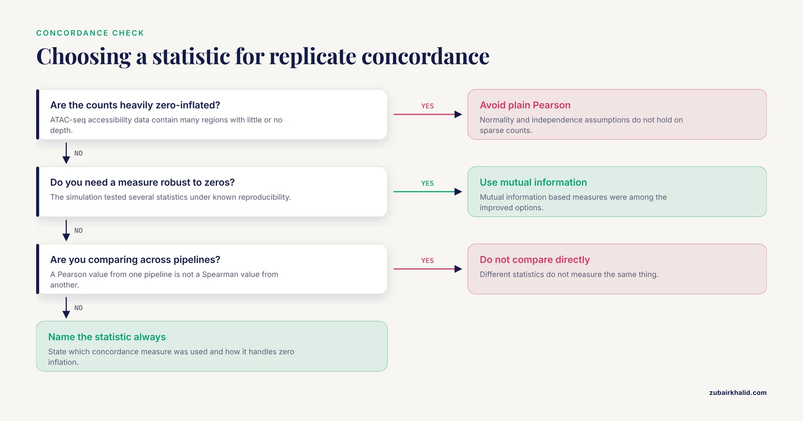
When you compare two replicates, the instinctive move is to compute a Pearson correlation. For chromatin accessibility data such as ATAC-seq, that instinct is unreliable. Accessibility data across the human genome contain many regions with little or no sequencing depth, producing heavily zero-inflated distributions that violate the assumptions of normality, homoscedasticity, and independence that ordinary correlation carries with it.
Researchers built a computational simulation of ATAC-seq data to watch how Pearson R, Spearman rho, Kendall tau, Top-Down correlation, the coefficient of determination R squared, Kendall's W, and normalized mutual information behave when reproducibility conditions are known by construction. The experiments revealed insensitivity problems in some of the widely used statistics under the simulated conditions, and the authors argue for choosing association measures that handle the zero-heavy structure of the data, with mutual information-based measures among the improved options [7]. For the working analyst, the takeaway is concrete. When reporting replicate concordance for sparse genomic data, state which statistic you used, understand its behavior on zero-inflated data, and avoid comparing a Pearson value from one pipeline against a Spearman value from another as if they measured the same thing.
Microarrays and RNA integrity
Metric-based quality control predates high-throughput sequencing, and microarray data still teach the clearest lesson about the gap between a sample metric and a dataset metric. The RNA integrity number, RIN, is a sample-level metric computed from an electropherogram that summarizes RNA degradation on a 1 to 10 scale. The temptation is to discard every sample below some RIN cutoff.
A study of 34 Affymetrix Gene 1.0 ST array datasets from paired tumor and normal colorectal cancer samples showed why that temptation should be resisted. Seven arrays, 20.6 percent of the total, were flagged during array quality assessment, and those arrays came from samples with a mean RIN of 3.2. Yet ten arrays from samples with RIN values below 7 passed quality assessment, including one sample with a RIN below 3. Transcript-length bias from RNA degradation appeared in only 5.8 percent of annotated transcript clusters under the criteria tested. The practical conclusion is that sample integrity and array quality are related but distinct, that quality-flagged arrays and degraded-RNA arrays do not fully overlap, and that analysts should use within-array and between-array measures rather than relying on RIN alone [8]. This is one of the cleanest demonstrations in the literature that genomics data quality metrics interpretation requires knowing what each metric actually measures.
Single-cell and spatially resolved data
Single-cell genomics produces per-cell metrics such as total counts, the number of detected genes, and the percentage of mitochondrial counts. Cells failing these metrics are conventionally filtered before analysis. The subtlety appears when the data have spatial structure, because a global threshold applied across a whole tissue section can remove cells that are perfectly healthy but sit in a tissue region with naturally different properties.
Spatially aware quality control solves this by computing neighborhood-aware z-scores. A cell is flagged as an outlier only relative to its local spatial neighborhood, not relative to the entire section. SpotSweeper introduced this approach in R, and SpotSweeper-py brings the same neighborhood-aware z-scores for total counts, log total counts, number of detected genes, and percentage of mitochondrial counts into the Python and scverse ecosystem, with plotting utilities for visualizing flagged outliers. Demonstrations on 10x Genomics Visium and VisiumHD datasets showed that local metrics reduce false positives from global quality control while preserving tissue-specific architecture [9].
The scale of the filtering decision is visible in a real study. In a project combining CosMx high-plex spatial transcriptomics with whole-genome-sequenced colorectal cancer samples from the Genomics England 100,000 Genomes Project, 966,500 cells were detected before quality control across 65 tissue microarray cores on three slides, and 935,262 high-quality cells were retained after multistep quality control before cell typing, pathway enrichment, spatial neighborhood analysis, and regulatory network inference [10]. Roughly 3 percent of detected cells were removed, a reminder that sensible QC should trim a small tail, not decimate the dataset.
Domain-specific variants of these metrics are emerging where the biology demands them. A quality control toolkit for single-cell epigenomic data from CAR-engineered T cells combines standard single-cell assay metrics, FRiP and TSS enrichment, with detection of signal from CAR vector insertion sites, supporting 10x Genomics and non-10x data formats and producing summary outputs suited to regulatory-grade preclinical reporting [11]. The lesson generalizes. When an experiment has a designed feature that standard metrics cannot see, quality control has to be extended to see it.
Variant data and read depth
For germline variant interpretation, the central quality question is whether the sequencing depth of the data supports the claims made about allele frequencies and variant calls. A simulation study generated germline genome sequence data at nine read depths and found that a 30X read depth achieved acceptable precision and recall for detecting substitutions, but recall for small insertions and deletions remained poor even at that depth. Examining population frequency resources, the same work found that exome-derived and genome-derived datasets showed low read depth for different gene exons, and that applying a minimum acceptable read-depth threshold resolved divergent allele frequency classifications for some variants in cancer syndrome genes [12]. Two lessons follow. Read-depth requirements differ by variant type, so a depth that is adequate for single-nucleotide variants is not automatically adequate for indels. And population frequency data should be assessed for sequencing quality metrics before being used in variant interpretation, rather than treated as context-free ground truth.
Association study data
Genome-wide association studies bring their own quality demands, centered on per-marker and per-sample call rates, Hardy-Weinberg expectations, population structure, and batch consistency. A dedicated data quality framework for GWAS framed these requirements explicitly as a data quality problem, with measurable attributes and enforcement at the dataset level rather than as informal lab habits. The GWAS framing is useful beyond association mapping, because it treats every dataset as having quality dimensions that can be defined, measured, and audited, the same posture that underlies modern bioinformatics data management.
How Quality Metrics Are Interpreted in Practice
Metrics acquire meaning through three mechanisms, and a working bioinformatician should be fluent in all three.
The first mechanism is comparison within a project. Outlier detection asks whether one sample departs from the distribution of its peers. In the proficiency-testing study described above, 11 percent of genomes were identified as outliers in at least one QC metric and excluded from the computation of adjusted quality thresholds, a deliberate two-step design where outliers are removed before thresholds are set so that extreme values do not inflate the limits for everyone else [5].
The second mechanism is correlation among metrics. The same study identified two correlation groups among its QC metrics, meaning sets of metrics that rise and fall together, and used uncorrelated metrics to identify genuinely underperforming laboratories. Eight percent of submitted genomes failed one or more of the adjusted quality thresholds, but only three of the 25 participating laboratories, 12 percent, failed across uncorrelated metrics on at least two genomes, distinguishing systemic underperformance from isolated bad runs [5]. This is a sophisticated point that applies far outside proficiency testing. If your QC panel contains five metrics that all measure the same underlying failure mode, four of them are redundant, and a sample that fails one will fail all. A well-designed panel spans independent failure modes.
The third mechanism is validation against an external standard. In clinical genomics, quality control metrics are chosen by testing the pipeline against real-world and synthetic data until its predictive performance is characterized, then accredited to international standards. A tuberculosis whole-genome sequencing pipeline built for clinical antimicrobial susceptibility prediction determined its quality control metrics through extensive validation before achieving accreditation suitable for clinical and public health microbiology laboratory settings, with the design kept flexible enough that non-programmers can tailor criteria to local needs [13]. This is the endpoint of the metrics lifecycle, where a number stops being advisory and becomes a release criterion.
Statistical benchmarking studies sharpen all three mechanisms. Work on visual quality metrics for high-dimensional genomic data connects computed metrics to human visual analysis, so that dimensionality-reduction plots can be judged with the same rigor as numeric summaries. Work on chemical genomics reanalysis found that no single best similarity metric exists for phenotypic profile comparison, with three tested metrics giving comparable results for most gene pairs, a finding that pushes analysts toward reporting multiple concordance measures rather than betting on one [14].
A Step-by-Step Quality Control Workflow
The most reliable way to make quality control reproducible is to fix the sequence of steps and record everything. The following workflow reflects standard practice across sequencing projects.
- Collect raw metrics at the source. Run per-file read QC on every FASTQ as it comes off the instrument. Capture per-cycle quality, GC content, adapter content, and duplication. Store these outputs, not just the summary verdicts, because raw reports can be reinterpreted later.
- Aggregate before judging. Combine per-sample reports into a project-level table so that batch patterns are visible. A metric that looks acceptable sample by sample can reveal a batch effect when tabulated across 96 libraries.
- Apply preprocessing and record it. Filter adapters, trim low-quality tails, remove blacklist regions where applicable, and mark or remove duplicates. Every one of these steps changes downstream metric values, as demonstrated for ChIP-seq and ChIP-exo metrics [6], so the report must state which preprocessing produced each number.
- Compute assay-specific metrics. Run the family that matches the data type, BUSCO for assemblies [2], strand cross-correlation and FRiP for ChIP [6], association measures suited to zero-inflated data for ATAC-seq replicates [7], per-cell metrics for single-cell and spatial data [9].
- Set thresholds from data, not folklore. Where established thresholds exist, use them. Where they do not, derive them from the distribution of your own samples, following the outlier-then-threshold logic used in proficiency testing [5], or from validation studies that tie thresholds to performance [13][12].
- Flag, do not silently delete. Record every excluded sample with the metric and value that excluded it. Silent removal is the single largest threat to reproducibility in quality control.
- Attach the metrics to the data. Persist the QC report alongside the dataset, in the same storage system, so that anyone who acquires the data years later can see how it was judged.
Governance, Annotation, and Storage
The infrastructure-policy dimension of quality metrics concerns what happens after the numbers exist. Three practices separate well-managed genomics data from ad hoc collections.
Standardized annotation of known issues. Public health laboratories increasingly need to share sub-optimal datasets for validation, training, and optimization, and these datasets are useful precisely because they contain known flaws. The PHA4GE quality control contextual data tags provide standardized attributes for annotating public health sequence datasets with known quality issues, so that such data can be identified in repositories, distinguished from better quality information, and reused appropriately rather than mistaken for clean data [3]. Without such tags, a dataset with a documented contamination event is indistinguishable from a pristine one to anyone who downloads it.
Traceable stewardship. Reviews of data stewardship in AI-based genomics and high-throughput imaging consolidate the requirements into a recognizable set, including data governance, quality management, privacy measures, access control, accountability, and traceability, all tied to curation frameworks and storage systems [4]. The practical translation is that every metric should be traceable to the pipeline, version, and parameters that produced it, because an untraceable metric cannot be audited and therefore cannot fully support a scientific or clinical claim.
Storage that preserves metrics. Genomics data storage policy should treat QC outputs as first-class objects. A FASTQ file without its QC report loses interpretive context, and a metric without the preprocessing record loses meaning. Facilities that expose quality metrics alongside data enable the cross-platform comparisons and data-driven informatics that improve experimental design over time [1]. For long-lived consortia, storing both raw QC reports and the derived summary tables, with timestamps and software versions, is the difference between a dataset that can be reevaluated and one that must be reprocessed from scratch.
Comparison With Adjacent Concepts
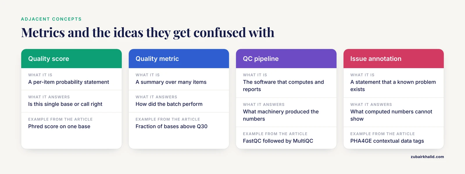
Genomics data quality metrics are frequently confused with three neighboring ideas, and the distinctions matter for correct interpretation.
A quality score is a per-item probability statement, such as the Phred score on a single base or a variant quality score on a single call. A quality metric is a summary over many items, such as the fraction of bases above Q30 or the mean depth across a gene. Both are needed, but they answer different questions. A quality control pipeline is the software system that computes metrics, applies thresholds, and produces reports. Metrics are the outputs. The pipeline is the machinery. A quality issue annotation is a human or standardized statement that a known problem exists in a dataset, which complements computed metrics because some failures, such as a swap of two sample labels, may never appear in any computed number [3].
Common Mistakes and Limitations
- Applying global thresholds to spatially structured data. Tissue-wide cutoffs on counts, detected genes, or mitochondrial percentage over-aggressively remove biologically meaningful regions or miss localized artifacts. Neighborhood-aware scores exist precisely because this failure mode is common.
- Comparing metrics across different preprocessing. An NSC computed before blacklist filtering is not comparable to one computed after, and benchmarking work shows the interpretation of ChIP-seq metrics shifts with the steps applied [6]. Always report the pipeline next to the number.
- Using sample metrics as dataset metrics. A RIN value describes RNA, not the array built from it. A meaningful fraction of low-RIN samples produced arrays that passed full quality assessment in the colorectal cancer study cited above [8]. Judge the data product with data-product metrics.
- Trusting Pearson correlation on sparse data. For ATAC-seq and similar zero-inflated count data, ordinary correlation statistics behave in ways their assumptions do not predict, and benchmarking shows some widely used statistics are insensitive under conditions of known reproducibility [7].
- Assuming one depth threshold fits all variant types. A 30X read depth achieved acceptable substitution detection in simulation but poor recall for small insertions and deletions [12]. Depth requirements are variant-type specific.
- Treating thresholds as universal. Species-specific thresholds for N50 and contig counts exist because a single number cannot serve 12 bacterial species with different genome architectures [5]. Adopting another lab's thresholds without checking the data type is a recurring failure.
- Discarding poor-quality data instead of annotating it. Datasets with known issues are essential for validation, training, and testing. Standardized contextual tags make them shareable and safe to reuse [3].
- Deleting outliers before computing thresholds. Thresholds set on data that include extreme values are inflated, which is why the proficiency-testing workflow excluded outlier genomes before computing adjusted thresholds [5].
- Leaving metrics out of storage and governance planning. Quality management, traceability, and curation frameworks are core components of stewardship for large genomics datasets, not optional extras bolted on at publication time [4].
Quick Review
- Genomics data quality metrics are repeatable measurements of completeness, accuracy, and fitness for a stated analysis, taken at every stage of the data lifecycle.
- Phred Q scores are logarithmic, so Q30 means an estimated 1 in 1,000 base error chance.
- Contiguity metrics such as N50 and completeness metrics such as BUSCO measure different failure modes and belong together [2].
- ChIP-seq metric values depend on preprocessing steps such as blacklist filtering and duplicate removal, so pipeline context must accompany every number [6].
- Zero-inflated data such as ATAC-seq accessibility violate ordinary correlation assumptions, and choice of concordance statistic changes the answer [7].
- Sample-level metrics such as RIN do not determine dataset-level quality, and low-RIN samples can pass array QC [8].
- Spatially aware neighborhood z-scores prevent global QC thresholds from removing valid tissue regions [9].
- Thresholds should be species, assay, and variant-type specific, derived from data or validation studies rather than folklore [13][12][5].
- Standardized annotation tags let datasets with known quality issues be shared and reused safely [3].
Frequently Asked Questions
What does genomics data quality metrics mean?
It means the set of standardized measurements taken on sequencing, array, or derived genomic data to judge whether the data are accurate, complete, and suitable for a given analysis. Examples include per-base Phred quality on reads, N50 and BUSCO completeness on assemblies, and per-cell counts and mitochondrial percentage on single-cell data.
Which metrics matter most for raw sequencing reads?
The core set is the per-cycle quality profile, per-base sequence content and GC distribution, adapter contamination, duplication level, and overrepresented sequences. Aggregating these across all samples in a project matters as much as the per-sample values, because batch-level patterns only appear when reports are combined.
What read depth is adequate for germline variant detection?
In simulation across nine read depths, a 30X read depth achieved acceptable precision and recall for detecting substitutions, while recall for small insertions and deletions remained poor. This means depth requirements depend on the variant type, and read depth should also be checked before using population frequency datasets in variant interpretation.
Why do quality thresholds differ between laboratories and species?
Genome size, repeat content, GC content, and assay design all shift the expected values of metrics such as N50 and contig count, so a single threshold cannot serve all species or all labs. Proficiency testing networks address this by resequencing shared isolates and publishing species-specific thresholds derived from real inter-laboratory data.
Can poor-quality genomics data still be useful?
Yes, when the problems are known and documented. Datasets with known quality issues are essential for validating pipelines, training staff, and testing assays. Standardized contextual annotation tags exist so these datasets can be shared in repositories, found by users, and interpreted without being mistaken for higher quality data.
How should quality metrics be stored and shared?
Store QC outputs alongside the dataset in the same storage system, with the pipeline version, parameters, and preprocessing steps recorded next to every metric value. Treat metrics as first-class metadata under a governance framework that includes traceability, access control, and curation, so any later user can audit how the data were judged.
Sources
- Sequencing quality assessment tools to enable data-driven informatics for high throughput genomics
- BUSCO: Assessing Genomic Data Quality and Beyond
- PHA4GE quality control contextual data tags: standardized annotations for sharing public health sequence datasets with known quality issues to facilitate testing and training
- Data stewardship and curation practices in AI-based genomics and automated microscopy image analysis for high-throughput screening studies: promoting robust and ethical AI applications.
- Whole-genome sequencing for antimicrobial surveillance: species-specific quality thresholds and data evaluation from the network of the European Union Reference Laboratory for Antimicrobial Resistance genomic proficiency tests of 2021 and 2022
- Impact of artifact removal on ChIP quality metrics in ChIP-seq and ChIP-exo data
- Improved quality metrics for association and reproducibility in chromatin accessibility data using mutual information
- Quality assessment and data handling methods for Affymetrix Gene 1.0 ST arrays with variable RNA integrity
- Spotsweeper-py: spatially-aware quality control metrics for spatial omics data in the Python ecosystem
- Abstract 65: Integrating spatial transcriptomics and digital pathology with whole-genome data from Genomics England to characterise the tumour and it's microenvironment in colorectal cancer.
- CARTEpigenoQC: A Quality Control Toolkit for CAR-T Single-Cell Epigenomic Data
- Considerations for using population frequency data in germline variant interpretation: Cancer syndrome genes as a model
- Bringing TB genomics to the clinic: A comprehensive pipeline to predict antimicrobial susceptibility from genomic data, validated and accredited to ISO standards
- Insights from the reanalysis of high-throughput chemical genomics data for Escherichia coli K-12