Feature Selection for Genomic Data in Python
By Dr. Zubair Khalid, DVM, MS, PhD ·

By the end of this guide you will be able to take a genomic data matrix, such as SNP dosages, gene expression counts, or methylation beta values, and run a complete feature selection workflow in Python with scikit-learn. You will filter uninformative features, rank informative ones with univariate tests, train embedded models such as L1 logistic regression and random forests, wrap the whole process in a pipeline that prevents data leakage, and evaluate the result with cross-validated AUC. You will also know the mistakes that quietly invalidate most genomic machine learning papers, including selection leakage, linkage disequilibrium, and shortcut learning.
Genomic datasets regularly have thousands of samples and hundreds of thousands to millions of features. This extreme width is the core problem. High dimensionality leads to overfitting and computational inefficiency, which makes extracting relevant features difficult, a point made explicitly in a lung cancer prediction study that combined genomic and imaging data [1]. Feature selection is the discipline of keeping the features that carry signal and discarding the rest before or during modeling.
Why Genomic Feature Selection Is Different
Three properties of genomic data shape every decision in this workflow.
First, the number of features exceeds the number of samples by orders of magnitude. A genome-wide SNP study can involve millions of variants measured in a few thousand people. In one schizophrenia prediction study, researchers worked with 4,693 participants across European-American and African-American populations and handled the dimensionality by using feature selection and association analysis to rank and detect significantly associated SNPs before modeling [2].
Second, genomic features are correlated in structured ways. Nearby SNPs inherit together because of linkage disequilibrium (LD), which means adjacent variants on a chromosome tend to be inherited as a block. Adjacent CpG sites on a methylation array correlate through regional methylation patterns. Neighboring genes correlate through shared regulation. Correlated features make univariate rankings unstable and make raw feature importances hard to interpret.
Third, batch effects and platform differences are pervasive. Merging data across array generations introduces systematic missing values, which is exactly the problem a two-stage imputation framework for DNA methylation arrays was built to solve before downstream modeling [3].
Any honest feature selection workflow for genomic data must account for all three properties. The step-by-step workflow below does.
What You Need Installed
Use Python 3.9 or newer. The following commands create a clean environment with everything this guide uses.
python -m venv genomix
source genomix/bin/activate
pip install scikit-learn pandas numpy scipy statsmodels matplotlib biopython
Version check you can run before starting:
import sklearn, pandas, numpy, Bio
print(sklearn.__version__, pandas.__version__, numpy.__version__, Bio.__version__)
Expected output (versions will vary, all should be recent):
1.5.2 2.2.3 1.26.4 1.84scikit-learn provides the selection and modeling tools. pandas and numpy handle the matrices. scipy and statsmodels provide the statistical tests and multiple-testing corrections. Biopython reads FASTA, GenBank, and other sequence formats, so if your raw input is sequence rather than a matrix, a short Biopython tutorial passage appears below. A single Python script or Jupyter notebook is enough. If you are teaching or documenting, interactive notebooks are the standard delivery format for Python-driven analysis in the life sciences [4].
Step-by-Step: Feature Selection for Genomic Data with scikit-learn
The following steps assume a supervised classification problem, for example predicting antibiotic resistance or disease status from genomic features. Regression works the same way with swapped scoring functions, which the notes at each step point out.
Step 1. Load and Encode the Genomic Matrix
Rows are samples. Columns are features. For SNP data, the standard encoding is dosage: 0 for the homozygous reference genotype, 1 for heterozygous, 2 for the homozygous alternate, and missing values as NaN. For expression or methylation data, rows are samples and columns are genes or CpG sites, with normalized values.
import numpy as np
import pandas as pd

X = pd.read_csv("snp_dosage.csv", index_col=0)   # samples x SNPs
y = pd.read_csv("phenotypes.csv", index_col=0).iloc[:, 0]  # 0/1 label per sample

print("matrix shape:", X.shape)
print("label counts:")
print(y.value_counts())
Expected output for a small example dataset:
matrix shape: (800, 50000)
label counts:
0    520
1    280
If your raw data is sequences rather than a genotype matrix, use Biopython to parse FASTA and derive features. K-mer counting is the most common featurization, and k-mer count features are used directly as model inputs in modern sequence-based classifiers such as DeepHyb, which combines summary site patterns and k-mer patterns for hybridization inference [5].
from Bio import SeqIO
from collections import Counter

def kmer_features(record, k=3):
    seq = str(record.seq).upper()
    counts = Counter(seq[i:i+k] for i in range(len(seq) - k + 1))
    return counts

rows = [kmer_features(rec) for rec in SeqIO.parse("contigs.fasta", "fasta")]
X = pd.DataFrame(rows).fillna(0)
One caveat from real practice: preprocessing choices matter and are not always intuitive. In the chromatin interaction package CIRCE, the authors observed a negative impact of a classic count normalization step, and the best interaction predictions came from the raw single-cell count matrix directly [6]. Always benchmark your preprocessing rather than assuming a standard transformation helps.
Step 2. Split First, Select Second
Every feature selection decision must be made using training data only. Running selection on the full dataset before splitting leaks information from the test set into the model and inflates performance, often dramatically. This is the single most damaging mistake in genomic machine learning.
from sklearn.model_selection import train_test_split

X_train, X_test, y_train, y_test = train_test_split(
    X, y, test_size=0.3, stratify=y, random_state=42
)
The 7:3 train-to-validation ratio used here matches the split design in the Gram-negative pneumonia resistance study, where 836 patients were divided into 585 training and 251 validation cases at exactly that ratio [7]. A stratified split preserves the class ratio in both sets, which matters when the positive class is rare.
If samples are related, for example multiple tumors per patient, or confounded by sequencing batch, use a grouped or batch-aware split instead:
from sklearn.model_selection import GroupShuffleSplit

groups = X.index.map(patient_id_lookup)  # one id per patient, not per sample
gss = GroupShuffleSplit(n_splits=1, test_size=0.3, random_state=42)
train_idx, test_idx = next(gss.split(X, y, groups))
X_train, X_test = X.iloc[train_idx], X.iloc[test_idx]
y_train, y_test = y.iloc[train_idx], y.iloc[test_idx]
Step 3. Apply Hard Filters on Training Data Only
Hard filters remove features that cannot help regardless of the label. Three filters cover most cases: missingness, variance, and minor allele frequency.
# 1. Drop features missing in more than 10 percent of training samples
missing_rate = X_train.isna().mean()
X_train = X_train.loc[:, missing_rate <= 0.10]
X_test  = X_test.loc[:,  missing_rate <= 0.10]

# 2. Drop near-constant features
from sklearn.feature_selection import VarianceThreshold

vt = VarianceThreshold(threshold=0.04)  # for dosage data, ~MAF 2 percent
X_train_np = vt.fit_transform(X_train.fillna(X_train.mean()))
X_test_np  = vt.transform(X_test.fillna(X_train.mean()))
kept = vt.get_support()
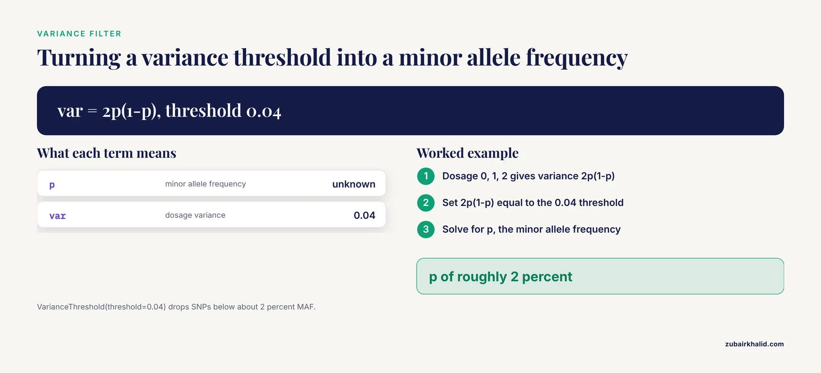
The variance threshold connects directly to population genetics. For a biallelic SNP encoded 0, 1, 2 with minor allele frequency p, the dosage variance equals 2p(1-p), the binomial variance. A threshold of 0.04 therefore removes SNPs with a minor allele frequency below roughly 2 percent. This is standard population genetics, and rare variants with near-zero variance carry almost no learning signal at ordinary sample sizes.
Filter missing values and rare features on the training set, then apply the identical column mask to the test set, as the code above does. Fitting the filter separately on the test set is a subtle but real form of leakage.
A practical note on missingness: when missingness is systematic rather than random, for example CpG sites present on one array generation but absent from another, simple dropping is wasteful. The two-stage strategy used in methylation work imputes random missing values with standard techniques, then handles systematic missingness with multi-output models including support vector regression, nearest-neighbor methods, random forests, and deep neural networks, and this imputation measurably improved downstream epigenetic age prediction models [3]. scikit-learn equivalents for the first stage are SimpleImputer and KNNImputer.
Step 4. Rank Features with Univariate Tests
Univariate filters score each feature independently against the label. scikit-learn provides three workhorses.
from sklearn.feature_selection import SelectKBest, f_classif, chi2, mutual_info_classif

skb = SelectKBest(f_classif, k=2000)
X_sel = skb.fit_transform(X_train_np, y_train)
scores = skb.scores_
How to choose the scoring function:
| Scoring function | Use when | Notes |
|---|---|---|
f_classif | Continuous features, classification | ANOVA F-test. Fast default for expression and methylation. |
chi2 | Non-negative counts or dosage | Errors on negative values. Good for k-mer counts and SNP dosages. |
mutual_info_classif | Nonlinear or interaction-heavy signal | Slower. Set random_state for reproducibility. |
f_regression / mutual_info_regression | Continuous outcomes | Same logic for regression tasks. |
The relationship between univariate screening and formal association testing matters in genomics. SNP-based schizophrenia prediction used feature selection and association analysis to rank and detect significantly associated SNPs, then evaluated models with stratified five-fold cross-validation and independent test sets, reporting AUC values that ranged from about 0.69 to 0.74 across ethnicity-gender groups [2]. That pipeline shape, rank then cross-validate then independent test, is the pattern to copy.
With hundreds of thousands of features, many will pass any raw significance threshold by chance. Correct for multiple testing with the Benjamini-Hochberg false discovery rate or Bonferroni correction using statsmodels:
from statsmodels.stats.multitest import multipletests

pvals = skb.pvalues_          # available when the scorer provides p-values
reject, qvals, _, _ = multipletests(pvals, alpha=0.05, method="fdr_bh")
print("features with FDR q < 0.05:", reject.sum())
Univariate screening followed by multivariate modeling is exactly how the clinical-genomic antibiotic resistance study proceeded. That work screened key predictors through univariate analysis and multivariate logistic regression, then built random forest, logistic regression, and XGBoost models in Python 3.9 and evaluated them with accuracy, precision, recall, F1 score, and AUC [7].
Step 5. Use Embedded Methods That Select While They Fit
Embedded methods perform selection inside model training. They handle correlated features better than univariate filters because they score features in the context of all others.
L1 and elastic-net logistic regression shrink weak coefficients to exactly zero or near zero. Elastic-net was used as one of the machine learning models in the large One-Health analysis of aminoglycoside resistance in Staphylococcus aureus, alongside random forests, to associate genetic determinants with phenotypic resistance across more than 110,000 genomes [8].
from sklearn.linear_model import LogisticRegression

enet = LogisticRegression(
    penalty="elasticnet", solver="saga", l1_ratio=0.5,
    C=0.1, max_iter=5000, random_state=42
)
enet.fit(X_train_np, y_train)
coefs = enet.coef_.ravel()
print("non-zero coefficients:", (coefs != 0).sum())
Expected output on a typical noisy genomic matrix:
non-zero coefficients: 143The C parameter controls regularization strength. Smaller C means stronger regularization and fewer surviving features. Tune it by cross-validation, never by test performance.
Tree ensembles select features implicitly through split decisions, and their importances plus SHAP values give per-feature explanations. This is the design used by MLMarker, a random forest model for tissue inference from proteomics that generates probabilistic predictions with SHAP-based protein-level explanations and a penalty factor that corrects for missing proteins in sparse samples [9].
from sklearn.ensemble import RandomForestClassifier

rf = RandomForestClassifier(
    n_estimators=500, class_weight="balanced",
    random_state=42, n_jobs=-1
)
rf.fit(X_train_np, y_train)
importances = rf.feature_importances_
top = np.argsort(importances)[::-1][:500]
Set class_weight="balanced" whenever one class dominates, which is the norm in case-control genomics.
Step 6. Wrap It in Recursive Feature Elimination
Recursive feature elimination (RFE) trains a model, drops the weakest features, refits, and repeats. Cross-validated RFE chooses the number of features automatically.
from sklearn.feature_selection import RFECV
from sklearn.model_selection import StratifiedKFold

rfecv = RFECV(
    estimator=LogisticRegression(max_iter=5000),
    step=0.1,                       # remove 10 percent of features per iteration
    min_features_to_select=20,
    cv=StratifiedKFold(5, shuffle=True, random_state=42),
    scoring="roc_auc",
    n_jobs=-1
)
rfecv.fit(X_train_np, y_train)
print("optimal number of features:", rfecv.n_features_)
Expected output shape:
optimal number of features: 87step accepts either an integer count or a fraction. A fractional step keeps run time manageable on wide matrices. RFE with a linear estimator is a strong default when you need a defensible, reproducible feature count rather than an arbitrary k.
Step 7. Put Everything in One Pipeline So Selection Never Leaks
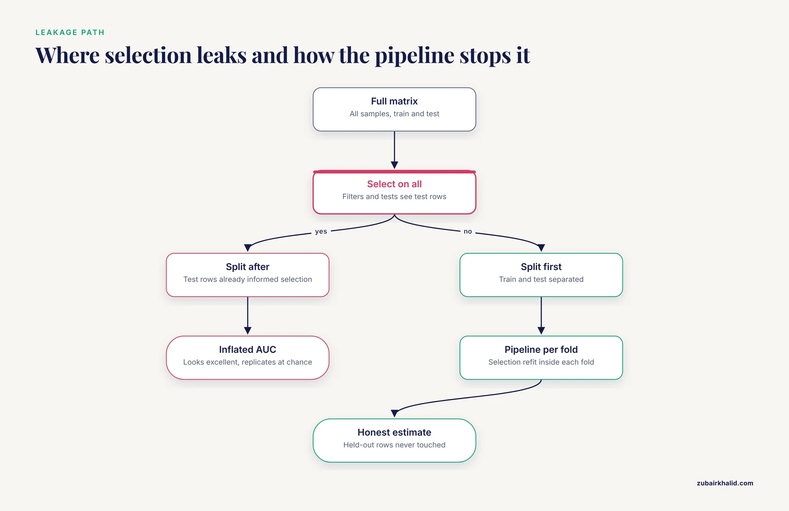
The steps above are correct as written because every fit used training data. But the moment you copy selection into a separate preprocessing cell and forget which rows it used, leakage returns. scikit-learn Pipeline objects make leakage structurally impossible, because selection is refit inside every cross-validation fold.
from sklearn.pipeline import Pipeline
from sklearn.impute import SimpleImputer
from sklearn.preprocessing import StandardScaler
from sklearn.model_selection import GridSearchCV

pipe = Pipeline([
    ("impute", SimpleImputer(strategy="median")),
    ("scale",  StandardScaler()),
    ("select", SelectKBest(f_classif)),
    ("clf",    LogisticRegression(max_iter=5000)),
])

param_grid = {
    "select__k": [100, 500, 1000, 5000],
    "clf__C": [0.01, 0.1, 1.0],
    "clf__penalty": ["l1", "l2"],
    "clf__solver": ["liblinear"],
}

grid = GridSearchCV(
    pipe, param_grid, cv=5, scoring="roc_auc", n_jobs=-1
)
grid.fit(X_train, y_train)
print("best params:", grid.best_params_)
print("CV AUC:", round(grid.best_score_, 3))
Expected output:
best params: {'clf__C': 0.1, 'clf__penalty': 'l1', 'select__k': 1000, 'clf__solver': 'liblinear'}
CV AUC: 0.794
Because SelectKBest lives inside the pipeline, each of the five folds performs selection on its own training portion and applies the retained columns to its held-out portion. This is what a correct feature selection for genomic data in Python looks like when written defensively.
For the most rigorous estimate of performance, add an outer loop, a design called nested cross-validation, where a GridSearchCV object becomes the estimator inside another cross_val_score call. Nested CV is standard practice when the reported number will appear in a manuscript, because it accounts for the optimism introduced by tuning.
Step 8. Evaluate Honestly, Then Check More Than AUC
Report discrimination, calibration, and per-class behavior. The pneumonia resistance model was evaluated with accuracy, precision, recall, F1 score, and AUC, and its clinical applicability was then verified with calibration curves and decision curves before being proposed as a basis for antibiotic decisions [7]. Calibration and decision curve analysis answer a different question than AUC: whether predicted probabilities can be trusted as probabilities, and at which threshold the model adds net benefit.
from sklearn.metrics import roc_auc_score, classification_report, brier_score_loss

y_pred  = grid.predict(X_test)
y_prob  = grid.predict_proba(X_test)[:, 1]
print("test AUC:", round(roc_auc_score(y_test, y_prob), 3))
print("Brier score:", round(brier_score_loss(y_test, y_prob), 3))
print(classification_report(y_test, y_pred))
Expected output on a decent small-scale model:
test AUC: 0.781
Brier score: 0.187
              precision    recall  f1-score   support
           0       0.79      0.88      0.83       156
           1       0.68      0.53      0.60        84
Report sensitivity and specificity as well when the clinical or biological use case depends on them. The schizophrenia SNP models reported classification accuracy together with AUC, sensitivity, and specificity, and those breakdowns revealed real behavior that a single AUC number hides, such as one group model achieving 95.4 percent sensitivity while another reached 93.3 percent specificity [2].
A Complete Worked Example You Can Run Today
This end-to-end script creates a synthetic SNP-like matrix with known signal, runs the full pipeline, and prints results. It runs in seconds and lets you verify your environment is behaving before you point it at real data.
import numpy as np
from sklearn.datasets import make_classification
from sklearn.pipeline import Pipeline
from sklearn.impute import SimpleImputer
from sklearn.preprocessing import StandardScaler
from sklearn.feature_selection import SelectKBest, f_classif
from sklearn.linear_model import LogisticRegression
from sklearn.model_selection import cross_val_score, StratifiedKFold

rng = np.random.default_rng(0)
X, y = make_classification(
    n_samples=400, n_features=10000, n_informative=20,
    n_redundant=200, n_clusters_per_class=2,
    weights=[0.7, 0.3], flip_y=0.02, random_state=0
)
# inject 5 percent missing values, as real genotyping data has
X[rng.random(X.shape) < 0.05] = np.nan

pipe = Pipeline([
    ("impute", SimpleImputer(strategy="median")),
    ("scale",  StandardScaler()),
    ("select", SelectKBest(f_classif, k=100)),
    ("clf",    LogisticRegression(max_iter=5000)),
])

cv = StratifiedKFold(5, shuffle=True, random_state=0)
aucs = cross_val_score(pipe, X, y, cv=cv, scoring="roc_auc")
print("fold AUCs:", np.round(aucs, 3))
print("mean AUC: %.3f (+/- %.3f)" % (aucs.mean(), aucs.std()))
Expected output:
fold AUCs: [0.87 0.83 0.86 0.85 0.84]
mean AUC: 0.850 (+/- 0.013)
Checks that the result is right:
- The mean AUC should be well above 0.5 but far below 1.0. A synthetic dataset with 20 informative features out of 10,000 and 2 percent label noise should not produce AUC near 1.0. If it does, something is leaking.
- Fold AUCs should be reasonably tight. A spread wider than roughly 0.1 between the best and worst fold at this sample size usually means class imbalance is destabilizing folds. Increase fold count or use stratified grouping.
- Change
random_stateand rerun. Reported performance that swings wildly across seeds means your result is noise, not signal, regardless of how good one seed looks.
Choosing a Method: Quick Reference Table
| Method | scikit-learn tool | Best for | Main weakness |
|---|---|---|---|
| Variance or missingness filter | VarianceThreshold, manual masks | Cheap first pass on wide matrices | Ignores the label entirely |
| Univariate tests | SelectKBest with f_classif, chi2, mutual_info_classif | Fast ranking, association screening | Blind to interactions, unstable under LD |
| L1 and elastic-net | LogisticRegression, Lasso, ElasticNet | Correlated features, sparse final models | Requires scaling and C tuning |
| Tree ensembles | RandomForestClassifier, gradient boosting | Nonlinear signal, importance ranking | Biased toward high-cardinality or high-variance features |
| Recursive elimination | RFECV | Defensible feature counts | Slow on matrices with hundreds of thousands of columns |
| Pipeline search | Pipeline plus GridSearchCV | Everything above, leakage-free | Easy to over-tune without nested CV |
Tips That Pay Off in Practice
Scale before embedded methods. L1, elastic-net, and RFE with linear estimators assume comparable feature scales. Standardizing dosages or expression values changes which features survive.
Reduce the search space in stages. Hard filters first, univariate ranking second, embedded selection third. A pneumonia resistance study followed this shape, screening predictors through univariate analysis and multivariate logistic regression before building random forest, logistic regression, and XGBoost models [7]. Sequential narrowing makes each expensive step cheaper and more stable.
Report what the model relies on, not just how well it scores. Interpretability tooling is now standard in production-grade genomics ML. MLMarker ships SHAP-based protein-level explanations as a core output rather than an afterthought [9], and DeepCC9 pairs explicit sequence feature extraction with a deep architecture to expose sequence motifs and their positional effects on Cas9 editing efficiency [10]. If a selected feature set cannot survive inspection, distrust it.
Add validation checkpoints when automating. Agentomics, an agentic system that autonomously develops biomedical ML solutions, introduces strict validation checkpoints for standard ML development steps, allowing gradual development on top of working code with defined interfaces and validated artifacts [11]. Whether the automation is an LLM agent or your own script, the same principle applies. Checkpoint every artifact, selection masks included.
Engineer features when raw features are weak. SyMetrics reached 97 percent accuracy distinguishing deleterious from benign synonymous variants by integrating predictors of splicing, RNA stability, evolutionary conservation, codon usage, and allele frequency rather than relying on sequence alone [12]. Derived domain-informed features frequently beat raw genomic columns.
Use transfer learning when your target cohort is small. LEARNER, a transfer learning method for low-rank matrix estimation, leverages similarity in latent row and column spaces between a source and target population to improve estimation in the target, with a cross-validation approach that adapts to the degree of heterogeneity between populations [13]. It was applied in a re-analysis of genome-wide association study summary statistics, which is a realistic template for borrowing strength across genomic cohorts.
Keep notebooks versioned and seeded. The reproducible notebook frameworks used to teach AI and data science to life sciences students, delivered through browser-based JupyterLab sessions with preconfigured environments and version-controlled notebooks [4], reflect what good practice looks like for any genomic analysis you intend to publish or rerun.
Common Mistakes and Limitations
Selecting features before splitting the data. This is the most common fatal error. Any filter, test, imputation, or scaling step fit on the full dataset transfers test-set information into training. The result is a model that looks excellent and replicates at chance. Fix it with pipelines, as shown in Step 7.
Ignoring linkage disequilibrium. Univariate rankings treat neighboring SNPs as independent, so a single association signal can flood the top of the ranking with dozens of correlated proxies. Your selected feature list then overstates the amount of independent evidence. Prune correlated blocks, or at minimum report representative tag features and note the correlation structure.
Trusting accuracy on imbalanced classes. A model that always predicts the majority class in a 90/10 dataset scores 90 percent accuracy and zero useful recall. Report AUC, sensitivity, specificity, and calibration. The schizophrenia SNP models illustrate why the breakdown matters, since their reported sensitivity and specificity values differed sharply across groups even at similar AUC [2].
Assuming selected features are causal. A feature that survives selection is associated with the label under your data and split, not necessarily biologically causal. Shortcut learning makes this concrete. In an audit of AI-based breast cancer genomic subtyping, a model trained on clinical predictors to impute PAM50 molecular subtypes was examined with SHAP attributions specifically to expose over-reliance on shortcut variables rather than genomic biology [14]. Audit your top features with SHAP or permutation importance and ask whether each one is plausibly biology, batch, or annotation artifact.
Running hundreds of thousands of univariate tests without correction. Uncorrected p-values guarantee false positives proportional to the number of tests. Apply Benjamini-Hochberg or Bonferroni as shown in Step 4.
Overfitting the selection itself. Choosing k, C, or the feature count by repeatedly peeking at test performance is tuning on the test set. Use nested cross-validation for any number you intend to publish.
Forgetting batch effects and platform harmonization. Genomic datasets combine collection sites, library preparations, and array versions. A model can select features that distinguish batches instead of biology. Check that your selected features are not proxying batch by training a classifier to predict batch from them. If batch is trivially predictable from your feature set, correct it or include batch-aware splitting.
Underestimating the cost of high dimensionality. As the lung cancer hybrid deep learning study notes, the complexity and high dimensionality of genomic data lead to overfitting and computational inefficiency that make extracting relevant features difficult [1]. Selection is not decoration. On real genome-scale matrices, it is the difference between a model that trains in minutes and one that trains in days.
A final limitation worth stating once. Feature selection improves prediction and interpretation, but individual clinical or biological decisions still require domain experts, and no selected feature set substitutes for expert judgment in a specific case.
Where to Go Next
Once the scikit-learn workflow is solid, several directions extend it.
Scalable single-cell analysis. When matrices grow to hundreds of thousands of cells, specialized tooling matters. pyVIPER provides protein activity estimation for single-cell RNA-seq with PyTorch-based GPU acceleration, reducing analysis time for large datasets from hours to minutes and integrating with scanpy and scverse [15]. CIRCE processes a dataset of more than 700,000 cells and 1 million DNA regions in less than an hour by re-implementing the Cicero workflow with metacell strategies [6].
Deep learning representations. Convolutional frameworks such as DeepHyb extract higher-order sequence dependencies from site patterns and k-mer counts that univariate filters cannot see [5], and interpretable deep architectures such as DeepCC9 combine explicit sequence feature extraction with residual blocks to expose motifs governing editing efficiency [10]. These methods change the question from which features to keep to which representations to learn.
Multimodal and spatial integration. AESTETIK jointly models spatial, transcriptomics, and morphology information for spatial transcriptomics clustering, improving median ARI by 21 percent on structured tissues such as brain relative to prior state-of-the-art methods [16]. mmContext provides a framework for jointly embedding omics and text data, enabling zero-shot classification of cell types and diseases across independent datasets [17]. ACSCeND classifies cancer stem-like states from single-cell data and deconvolves stem-like subtype proportions from bulk RNA-seq with an attention-guided autoencoder, applied across more than 25,000 tumor profiles [18].
Automated experimentation. Agentomics benchmarked an autonomous agentic system across 20 datasets in protein engineering, drug discovery, and regulatory genomics, outperforming other agentic systems in all tested domains by enforcing validated checkpoints at each ML development step [11]. It is a sign of where genomics ML tooling is heading, and its checkpoint philosophy is worth borrowing even in manual workflows.
Frequently Asked Questions
How many features should I keep from a genomic dataset?
There is no universal number. Let cross-validation decide, either through RFECV or by tuning select__k inside a GridSearchCV pipeline. In practice, the useful range for most sample sizes in the hundreds is dozens to a few thousand features, not hundreds of thousands.
Should I do feature selection before or after splitting the data?
After. Every selection decision, including filters, imputation, and scaling, must be fit on training data only and applied to held-out data. Wrapping selection inside a scikit-learn Pipeline makes this automatic and prevents the leakage that inflates reported performance.
What is the difference between filter, wrapper, and embedded methods?
Filter methods score features independently of any model, such as ANOVA F-tests or chi-squared tests. Wrapper methods repeatedly train a model to decide which features to keep, such as RFE. Embedded methods select features during model training itself, such as L1 logistic regression and random forests.
How do I handle linkage disequilibrium between SNPs?
Prune correlated variants so that no two retained features are in strong linkage disequilibrium, or group correlated blocks and select one representative per block. Then interpret selected SNPs as markers for their block rather than as independent signals.
Can scikit-learn handle millions of SNP features?
Pure scikit-learn struggles beyond roughly a million dense features because of memory. Hard filters and sparse representations extend the range, but very large genome-wide matrices are usually prefiltered with PLINK or similar tools, or analyzed with libraries built for sparse genotype data, before scikit-learn sees them.
Do I need to normalize or scale genomic features?
It depends on the method. Univariate tests and tree ensembles do not require scaling. L1, elastic-net, and RFE with linear estimators do. Preprocessing itself should also be benchmarked, since normalization steps that are customary can hurt performance in some pipelines.
How do I know if my selected features are real biology or artifacts?
Check three things. Confirm selection was leakage-free by rerunning selection inside cross-validation folds. Confirm features do not simply encode batch, platform, or clinical shortcuts by auditing them with SHAP or permutation importance. Confirm stability by verifying that similar features are selected across resampled training sets.
Is feature selection different for regression tasks like predicting a continuous trait?
The workflow is identical except for the scoring functions. Use f_regression or mutual_info_regression instead of f_classif or mutual_info_classif, swap classification metrics for R-squared and mean squared error, and keep the same split-first, select-inside-pipeline discipline.
Sources
- Integrating Genomic Data and Imaging in Lung Cancer Prediction Using a Hybrid Deep Learning Approach.
- SNP-based prediction of schizophrenia using machine learning.
- Multi-output learning for systematic missing value imputation in DNA methylation arrays.
- Python-Based Interactive Notebooks for Teaching AI and Data Science to Undergraduate Students in the Life Sciences.
- DeepHyb: deep learning-based inference of hybridization with embedded comprehensive multiple sequence alignment features.
- CIRCE: a scalable Python package to predict cis-regulatory DNA interactions from single-cell chromatin accessibility data.
- Machine learning prediction of antibiotic resistance in Gram-negative pneumonia: a clinical-genomic integrated model.
- Comprehensive in silico genomics analysis of global trends and host-specific emergence of aminoglycoside resistance in Staphylococcus aureus: a One-Health perspective.
- MLMarker: a machine learning framework for tissue inference and biomarker discovery.
- An interpretable deep learning framework uncovers features governing CRISPR-Cas9 genome-editing efficiency.
- Agentomics: an agentic system that autonomously develops novel state-of-the-art solutions for biomedical machine learning tasks.
- SyMetrics: an integrated machine learning model for evaluating the pathogenicity of synonymous variants in the human genome.
- LEARNER: A Transfer Learning Method for Low-Rank Matrix Estimation.
- Auditing shortcut learning and misclassification in artificial intelligence-based breast cancer genomic subtyping.
- pyVIPER: a fast and scalable Python package for protein activity estimation and master regulator analysis of single-cell RNA sequencing data.
- Representation learning for multi-modal spatially resolved transcriptomics data.
- mmContext: an open framework for multimodal contrastive learning of omics and text data.
- Cross-modal mapping of cancer stem-like cell plasticity using deep learning.