Bioinformatics Tool Evaluation Checklist: Template and Examples
By Dr. Zubair Khalid, DVM, MS, PhD ·

By the end of this article you will be able to take any bioinformatics tool, run it through a structured evaluation checklist, score it against your own requirements, and document the decision well enough that a colleague can reproduce it. You will need a candidate tool, a small representative test dataset, a way to run isolated environments (conda or Docker), a spreadsheet or plain-text file for scoring, and about a day of hands-on work for a serious evaluation. A quick triage pass takes about an hour.
The checklist below is built around the same dimensions that published benchmarking studies use when they compare tools head to head. Those studies exist because the field is crowded. A recent review of phage bioinformatics counted more than 80 dedicated tools, most published since 2020, spanning identification, assembly, annotation, taxonomy, and host prediction [1]. Benchmarking of structural variant callers evaluated 14 high-performing tools against a pedigree-based truth set and found substantial performance differences driven by underlying algorithm choice [2]. When the choice between two tools can change your biological conclusions, picking on reputation or download counts alone is a recipe for wasted compute and wrong answers.
Why Formal Tool Evaluation Matters
Three trends make a written checklist worth the effort.
First, tool volume keeps growing faster than anyone can test by hand. The phage bioinformatics literature now spans three successive computational paradigms, sequence homology, machine learning, and foundation models, each with different dependencies on database completeness and labeled training data [1]. A tool that looks state of the art may inherit every weakness of the database underneath it.
Second, headline benchmark numbers rarely transfer cleanly to your data. A systematic evaluation of ambient RNA decontamination tools for single-cell RNA sequencing showed that the tools have distinct strengths, so the right choice depends on data characteristics and research goals rather than a single global winner [3]. The same pattern appears in peptide-HLA binding prediction, where 17 models evaluated on a curated dataset of over 290,000 peptides across 44 HLA-I alleles showed substantial performance disparities, and models trained on eluted ligand data outperformed models trained on binding affinity data [4]. Training data provenance changed the ranking.
Third, reproducibility in published computational work remains poor. A systematic review of artificial intelligence in neurodegenerative diseases screened 4,685 records, included 1,186 studies, and found a reproducibility rate of only 35 percent, with external validation rarely using geographically or demographically diverse datasets [5]. If the field at large documents tool choices this loosely, your own written record is what keeps a pipeline auditable six months later.
The Bioinformatics Tool Evaluation Checklist Template
The template has twelve categories. Score each item 0 (fail or unknown), 1 (partial), or 2 (strong). Copy this into a text file or spreadsheet and fill one column per tool. This is the bioinformatics tool evaluation checklist format I use for pipeline decisions, and it maps directly onto the dimensions published benchmarks actually measure.
Category 1: Task and Data Fit
- Does the tool solve exactly your problem, not an adjacent one?
- Does it accept your input format natively (FASTQ, BAM, VCF, h5ad, FASTA, mzML)?
- Is it designed for your organism, data type, or scale, or is that an assumption you have to test?
- Has anyone demonstrated it on data like yours (tissue, species, sequencing platform, sample size)?
Category 2: Scientific Basis
- What paradigm does the tool use, and what are that paradigm's known limits? Sequence homology methods are bounded by database completeness, machine learning methods by labeled training data, and newer foundation-model approaches by both [1].
- What reference data, model weights, or databases does it ship with or download?
- Is the algorithm described in a peer-reviewed publication with methods you can read?
Category 3: Published Performance Evidence
- Do the authors report metrics on data independent of their training set?
- Are the metrics appropriate (see the metrics table below)?
- Is there an independent benchmark that includes this tool, not just the authors' own comparison?
Category 4: Benchmark Independence and Overfitting Risk
- Was the evaluation dataset plausibly used during tool development? A recent structural variant benchmark chose a newly released pedigree-based truth set specifically to minimize the chance the data had been used for training, reducing overfitting risk [2].
- For machine learning tools, is the training/test split described, including homology-based leakage control where relevant?
Category 5: Accuracy Metrics You Can Recompute
- Does the tool or its benchmark provide a truth set, simulated data, or gold-standard comparison you can rerun?
- Can you compute precision, recall, and F1 yourself from the outputs?
Category 6: Reproducibility and Provenance
- Is the exact version pinned (release number, commit hash, container digest)?
- Does the tool record parameters, input checksums, and versions in its output or logs?
- Reviews of agentic and AI-driven bioinformatics systems note that safeguards such as sandboxed execution, restricted commands, interaction logs, and evidence identifiers exist, but published reports rarely connect the biological question through samples, decisions, and validation in one traceable account [6]. A tool that logs its own provenance is easier to defend.
- Is random seed control available for stochastic methods?
Category 7: Dependencies and Shared Infrastructure
- What does the tool depend on (specific aligners, gene callers, protein language models, structural search backends)?
- Reviews of upstream components in phage bioinformatics, including gene callers, homology engines, protein language models, and structural search tools, expose shared infrastructure and ecosystem-level fragility when those dependencies change [1]. If three of your candidate tools all wrap the same upstream aligner, they share that failure mode.
- Are dependencies installable in an isolated environment without version conflicts?
Category 8: Resource Requirements
- Wall-clock time and peak memory on a dataset sized like yours?
- GPU required or optional?
- Does it parallelize across samples or nodes?
Category 9: Usability and Interface
- Command line, web server, or both? A web tool such as MARCo, which provides interactive scatter plots, correlation statistics, and heatmap modules over a dataset of 70,955 single-antigen bead results, trades pipeline automation for accessibility and visualization [7]. Decide which trade you need.
- Are the documentation and error messages usable?
- Is there an active issue tracker or support channel?
Category 10: Output and Interoperability
- Does it emit standard formats (VCF, GFF3, BIOM, h5ad, Newick) or bespoke ones?
- Can downstream tools in your pipeline consume it without custom parsing?
- Does frequency filtering or post-processing exist to keep the interpretation load manageable? In the structural variant benchmark, frequency filtering cut the downstream variant interpretation load by nearly half [2].
Category 11: Interpretability
- For prediction tools, can you inspect why a prediction was made? Explainability techniques such as SHAP and LIME were used to dissect the prediction mechanisms of HLA-I binding models, and ensemble or multi-algorithm approaches improved reliability [4].
- Reviews of machine learning in genome-wide association studies flag interpretability and the curse of dimensionality as key issues that separate useful models from black boxes [8].
Category 12: Maintenance and Sustainability
- When was the last release or commit?
- Is there a license that fits your use (academic, commercial)?
- Is the tool cited and reused by others, or is it a single-paper artifact?
Checklist Scoring Format
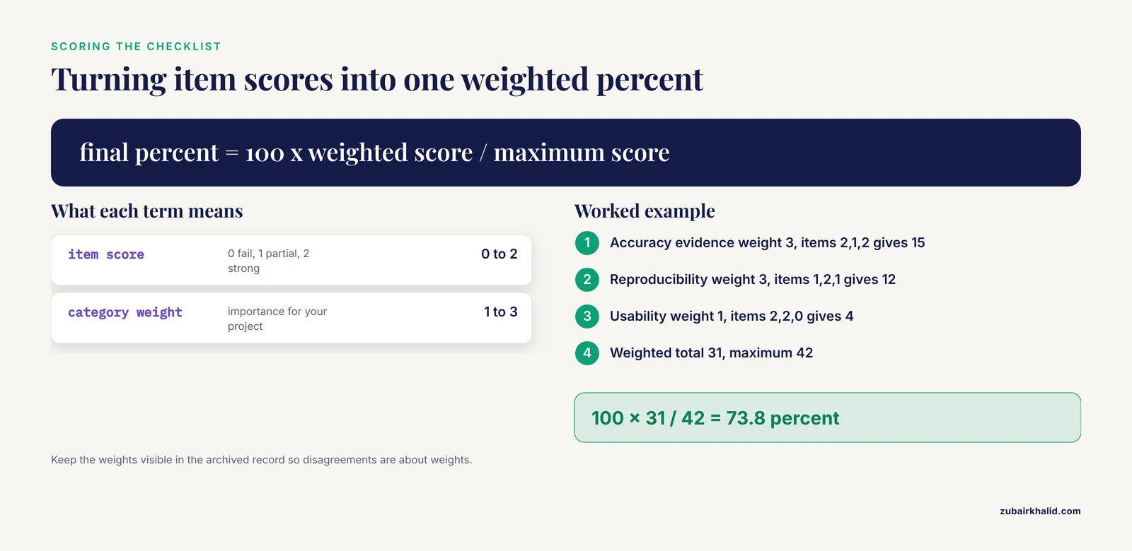
A simple weighted format keeps the math honest and fast.
- Assign each category a weight from 1 to 3 based on how much it matters for your project. For a clinical pipeline, reproducibility and accuracy evidence get weight 3. For an exploratory scan, usability can carry more weight.
- Score each item 0, 1, or 2.
- Compute the weighted total and normalize to a 0 to 100 scale.
The formula:
weighted score = sum(item score x category weight)
maximum score  = sum(2 x number of items x category weight)
final percent  = 100 x weighted score / maximum score
Worked example with three categories:
Accuracy evidence:    weight 3, items scored 2,1,2  -> (2+1+2) x 3 = 15
Reproducibility:      weight 3, items scored 1,2,1  -> (1+2+1) x 3 = 12
Usability:            weight 1, items scored 2,2,0  -> (2+2+0) x 1 = 4
Weighted total  = 31
Maximum         = (6 x 3) + (6 x 3) + (6 x 1) = 42
Final percent   = 100 x 31 / 42 = 73.8
Structured scoring instruments are standard practice in adjacent fields. Comparative reviews in analytical chemistry apply named metrics such as SPMS, NQS, SAMI, and the SIX Score to turn qualitative judgments into objective, data-driven scores [9]. The same discipline transfers to bioinformatics tool comparison, and the template above is your version of it.
Worked Walkthrough: Evaluating a Candidate Tool
The following walkthrough uses a hypothetical command-line tool called variantx. Every command shown is standard and works for any similar CLI tool. Adapt names and paths.
Step 1: Capture Version and Provenance First
variantx --version
variantx --help > variantx_help.txt
conda list -n variantx-env > variantx_packages.txt
Expected output for the first command:
variantx 1.4.2 (build 8f3a1c2)If the tool prints no version, that is an automatic score of 0 for the reproducibility category. Version ambiguity is the single most common reason an evaluation cannot be reproduced later.
If you install with conda, export the full environment so the evaluation is rerunnable:
conda env export -n variantx-env > variantx_env.ymlExpected output (truncated):
name: variantx-env
channels:
  - conda-forge
  - bioconda
dependencies:
  - python=3.11
  - variantx=1.4.2
If you install with Docker, record the digest, not just the tag:
docker inspect --format='{{index .RepoDigests 0}}' variantx/variantx:1.4.2Expected output:
variantx/variantx@sha256:3d9f...a41cStep 2: Build or Obtain a Test Dataset
Use something small, representative, and, if possible, paired with known answers. Published benchmarks are good sources of truth sets. The structural variant benchmark used four samples from a newly published, high-confidence pedigree-based truth set plus an in-house dataset [2]. Simulated data are another legitimate option, and the epistasis evaluation used the EpiGEN simulator to generate synthetic datasets modeling four classes of pairwise SNP interactions, dominant, multiplicative, recessive, and XOR [10].
If you simulate, keep the simulation parameters in the same directory as the results:
mkdir eval_variantx && cd eval_variantx
cp /data/truthset/sampleA.vcf.gz ./truth.vcf.gz
cp /data/truthset/sampleA.vcf.gz.tbi ./truth.vcf.gz.tbi
md5sum truth.vcf.gz > input_checksums.md5
Expected output of the last command:
d41d8cd98f00b204e9800998ecf8427e truth.vcf.gzYour hash will differ. The point is that the checksum file exists before you run anything.
Step 3: Run the Tool Under Controlled Conditions
Time it, measure memory, and capture stderr. The /usr/bin/time -v utility gives peak resident memory, which you need for the resource category.
/usr/bin/time -v variantx run --input sampleA.bam --reference GRCh38.fa \
  --output variantx_calls.vcf 2> variantx_run.log
Expected lines at the end of the log:
Elapsed (wall clock) time (h:mm:ss or m:ss): 0:14:22
Maximum resident set size (kbytes): 8412192
Exit status: 0
Record three numbers in the checklist: wall time, peak memory, and exit status. Exit status 0 means the tool believes it succeeded. Verify that belief in the next step.
Step 4: Inspect the Output Before You Trust It
Common failure modes are empty output, output in the wrong coordinate space, and headers that do not match your reference. Quick checks with standard tools:
ls -lh variantx_calls.vcf
grep -c "^#CHROM" variantx_calls.vcf
bcftools view -H variantx_calls.vcf | wc -l
bcftools stats variantx_calls.vcf > variantx_bcftools_stats.txt
head -40 variantx_bcftools_stats.txt
Expected output:
-rw-r--r-- 1 user user 4.2M Nov 11 09:31 variantx_calls.vcf
1
18457
If the variant count is 0 while the log says exit status 0, the tool silently failed. If the count is orders of magnitude higher than expected for your sample type, check whether the tool emitted every raw call with no filtering. In the structural variant benchmark, frequency filtering reduced the downstream variant interpretation load by nearly half before any biological interpretation happened [2]. Build that filtering step into your evaluation rather than judging the tool on raw output alone.
Step 5: Compare Against the Truth Set
For variant data, a matching step with standard tools gives you the counts you need for metrics:
bcftools isec -p isec_out -n=2 truth.vcf.gz variantx_calls.vcf
wc -l isec_out/0000.vcf isec_out/0002.vcf
0000.vcf holds positions present in both files. 0002.vcf holds positions unique to the tool. From the two counts you compute the core metrics (worked calculation in the next section).
For non-variant data, choose the comparison that matches the claim. When FTIR typing was evaluated against whole genome sequencing with bioinformatic comparison as the reference method for Serratia isolates, concordance was measured with the Adjusted Rand index and the Adjusted Wallace coefficient, yielding an Adjusted Rand index of 0.742, a positive predictive value of 0.842 for correctly identifying closely related isolates, and a negative predictive value of 1.0 for correctly identifying unrelated isolates [11]. The structure of that evaluation, a cheaper or faster method judged against a reference standard with concordance statistics, is exactly the pattern to copy for any classification or clustering tool.
Step 6: Stress Two Failure Directions
Run the tool once on degraded input and once on out-of-scope input, and record what happens:
# Degraded input: truncated file
head -c 1000000 sampleA.bam > truncated.bam
variantx run --input truncated.bam --reference GRCh38.fa --output t.vcf 2> degrade.log
echo "exit: $?"
Expected outcome, and what you want to see:
variantx: ERROR: truncated BGZF block in input BAM at offset 1000000
exit: 1
A loud failure with a nonzero exit code is good. A silent partial result with exit status 0 is a red flag worth a note in the checklist. Then run it on data outside its design range, for example a tiny sample or an organism it was not built for, and record whether it warns you or just produces output anyway.
Step 7: Score, Document, and Archive
Fill in one checklist column per tool, compute the weighted percent, and archive the directory:
tar czf eval_variantx_1.4.2.tar.gz eval_variantx/
sha256sum eval_variantx_1.4.2.tar.gz > eval_bundle.sha256
Expected output:
9f2b1c...e07a eval_variantx_1.4.2.tar.gzThe archive plus the completed checklist is your evaluation record. Anyone, including you in a year, can rerun the whole comparison.
Metrics Table: What to Compute and When
This table summarizes the key evaluation formulas. The definitions are standard, and the cited benchmarks use them in exactly these roles.
| Metric | Formula (plain text) | Use it when |
|---|---|---|
| , - | , - | , - |
| Recall (sensitivity) | TP / (TP + FN) | You cannot afford to miss true positives, as in pathogen or variant detection |
| Precision (PPV) | TP / (TP + FP) | False positives are costly, as in clinical interpretation workloads |
| F1 score | 2 x precision x recall / (precision + recall) | You need one balanced number across tools [2] |
| Specificity / NPV | TN / (TN + FN) | Confirming that negatives are truly negative, as in typing concordance studies [11] |
| MCC | (TP x TN - FP x FN) / sqrt((TP+FP)(TP+FN)(TN+FP)(TN+FN)) | Single balanced metric robust to class imbalance, reported in phage identification tasks above 0.95 for foundation models [1] |
| Adjusted Rand index | Chance-corrected agreement of two clusterings | Clustering or typing concordance against a reference method [11] |
| RMSD | sqrt(mean(distance squared between matched atom positions)) | Comparing a predicted structure to a reference structure [12] |
| Ramachandran statistics | Fraction of residues in favored, allowed, and outlier regions | Validating protein model stereochemistry, standard in homology modeling quality control [12] |
Worked metric calculation. Suppose a caller reports 120 structural variant calls against a truth set of 100 real variants, and 70 calls are true positives:
recall    = 70 / 100          = 0.70
precision = 70 / 120          = 0.583
F1        = 2 x 0.70 x 0.583 / (0.70 + 0.583) = 0.636
A recall of 0.70 on structural variants is actually high for short-read data. In the published benchmark, the best overall performer achieved a mean recall of 0.36 and mean F1 of 0.51, and among open-source tools Manta and Dysgu reached a mean recall of 0.26 with Manta at a mean F1 of 0.41 [2]. Knowing the realistic range from the literature keeps you from rejecting a good tool or, worse, trusting an implausibly perfect one.
Examples From Published Evaluations
These four published evaluations are the closest thing to filled-in checklists, and each one illustrates a different category doing real work.
Example: Matching Tool to Data Characteristics
The ambient RNA decontamination benchmark assessed seven tools using simulated and experimental datasets from diverse tissues and species, scoring accuracy in estimating contamination levels, robustness across conditions, and sensitivity to subtype-specific contamination [3]. The results were split rather than ranked. DecontX provided the most accurate contamination-level estimation. scAR was the most robust across conditions but tended to overestimate contamination. CellClear performed best for resolving closely related cell subtypes [3]. Checklist lesson: a category can have more than one winner, and your data characteristics decide which winner matters.
Example: Training Data Provenance Changes Rankings
In the peptide-HLA binding evaluation, the 17 models were assessed on accuracy, robustness, and interpretability over a curated dataset of more than 290,000 peptides across 44 HLA-I alleles [4]. Self-attention-based models including STMHCpan and BigMHC showed superior accuracy, the capsule network model CapsNet-MHC_AN was robust, and models trained on eluted ligand datasets outperformed those trained on binding affinity data [4]. Checklist lesson: two tools with identical architectures can rank differently because of training data, which is why the checklist separates scientific basis from performance evidence.
Example: Honest Reporting of Weak Performance
The epistasis detection evaluation tested six methods for quantitative phenotypes, including EpiSNP, Matrix Epistasis, MIDESP, PLINK Epistasis, QMDR, and REMMA, on EpiGEN-simulated datasets [10]. Performance varied by interaction type. REMMA achieved the highest overall detection rate at 55 percent and excelled on dominant interactions at 100 percent. MDR excelled on multiplicative at 57 percent and XOR at 69 percent. EpiSNP did best on recessive interactions at 67 percent. Critically, all methods except BOOST produced F1 scores below 0.05 for most interaction types [10]. Checklist lesson: publish-grade evaluations report the bad numbers, and an overall headline number can hide near-zero performance on the interaction types you care about.
Example: Protocol Variability as a Hidden Variable
A review of molecular docking studies of natural compounds as DPP-4 inhibitors evaluated more than 150 studies for docking methodology, protein structure selection, and validation strategy, and found substantial variability in computational protocols [13]. Many studies relied solely on docking results without further validation [13]. Checklist lesson: when you compare your results to published ones, the other authors' protocol choices are a hidden variable. Document your own choices (protein structure identifier, docking engine, scoring function, validation step) in the checklist record.
Example: Validation Metrics for Structural Predictions
The homology modeling literature defines a compact validation panel for structure prediction tools, covering template discovery with BLAST, model building with MODELLER or Swiss-Model, and structure validation with PROCHECK, ProSA, and VERIFY3D, using metrics including root mean square deviation, Z-score, and Ramachandran plot statistics [12]. Checklist lesson: for structure tools, the checklist items under accuracy metrics are already standardized. Adopt them rather than inventing your own.
Example: The Machine Learning Pipeline Audit
An integrative prostate cancer biomarker study built a stepwise, reproducible framework combining differential expression, pathway enrichment, protein-protein interaction networks, graph-convolutional feature selection, and a hybrid ensemble over Random Forest, Gradient Boosting Machine, Support Vector Classifier, Artificial Neural Network, and AdaBoost, with the algorithms systematically evaluated rather than assumed [14]. Checklist lesson: when a tool embeds machine learning, evaluate the modeling choices as part of the tool, and prefer pipelines that report the algorithm comparison itself.
Common Mistakes and Limitations
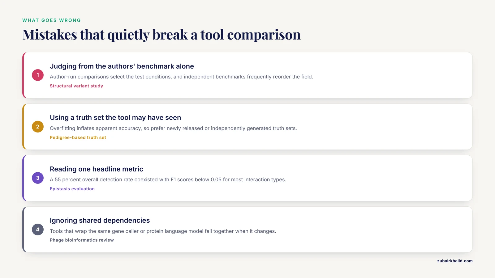
- Judging from the authors' benchmark alone. Author-run comparisons select the test conditions. Independent benchmarks frequently reorder the field, as the structural variant study did when it separated the best overall performer from the best open-source tools [2].
- Using a truth set the tool may have seen. Overfitting inflates apparent accuracy. Prefer newly released or independently generated truth sets, the explicit rationale in the pedigree-based truth set choice [2].
- Reading one headline metric. In the epistasis evaluation, a 55 percent overall detection rate coexisted with F1 scores below 0.05 for most interaction types across almost every method [10]. Check the metric breakdown against your interaction type, variant class, or cell subtype.
- Assuming a good tool transfers across data types. The ambient RNA study found winners that differed by tissue, species, and subtype structure [3]. Run the tool on a slice of your own data before committing.
- Ignoring shared dependencies. Tools that wrap the same gene caller or protein language model fail together when that upstream component changes, an ecosystem-level fragility documented in the phage bioinformatics review [1]. Note the upstream components in your checklist.
- Treating a prediction as validated. Docking reviews document many studies relying on docking scores alone without follow-up validation [13]. If your downstream decision is expensive, budget for experimental or orthogonal computational validation.
- Skipping version pinning. With a 35 percent reproducibility rate in AI-heavy biomedical research, unpinned versions are the difference between an auditable pipeline and an unreproducible one. Record version, container digest, and parameters every time.
- Overweighting ease of installation. Difficulty installing is a real cost but belongs in its own category. Do not let a smooth install substitute for accuracy evidence.
- Forgetting interpretability for ML tools. The GWAS machine learning literature emphasizes interpretability and dimensionality limits [8], and SHAP and LIME analyses are now practical for many model classes [4]. If you cannot explain a prediction to a collaborator, record that as a limitation in the checklist.
- Expecting any checklist to be complete. A checklist reduces, but does not eliminate, the risk that a tool behaves differently on your data at scale. Re-run the evaluation when data characteristics change materially.
One limitation of the checklist itself deserves a plain statement. Scores are judgments, and two evaluators can weight categories differently. Keep the weights visible in the archived record so disagreements are about weights, not hidden preferences.
Frequently Asked Questions
What is a bioinformatics tool evaluation checklist?
It is a structured list of criteria, covering task fit, accuracy evidence, reproducibility, resources, and maintenance, that you score a candidate tool against before adopting it. The scoring turns an opinion into a documented, comparable decision.
What metrics should I use to compare bioinformatics tools?
Use precision, recall, and F1 for detection tasks, Matthews correlation coefficient for imbalanced classification, Adjusted Rand index for clustering concordance, and RMSD with Ramachandran statistics for structure prediction. Match the metric to the type of error that would hurt your project most.
How many tools should I include in a bioinformatics tools comparison?
Include as many as you can run identically on the same test data, which for most lab projects means two to five candidates plus your current default. Published benchmarks handle larger fields, with examples evaluating 14 structural variant callers [2] and 17 HLA binding predictors [4].
Do I need a truth set to evaluate a tool?
You need some ground truth, but it can come from a published truth set, simulated data, or a reference method. The epistasis evaluation used simulator-generated datasets with defined interaction classes [10], and the FTIR study used whole genome sequencing results as the reference standard [11].
How do I evaluate machine learning based bioinformatics tools?
Check the training data provenance, ask whether your data resemble the training distribution, test whether explanations are available through methods such as SHAP or LIME, and prefer tools that report ensemble or multi-algorithm comparisons [4]. Beware training data leakage into the benchmark set [2].
What is the best bioinformatics software for my task?
The best tool is the one with the highest checklist score on the categories you weighted, validated on a slice of your own data. Published evaluations consistently show context-dependent winners rather than one overall best [3], so a tool ranked first in someone else's benchmark can rank third on your data.
Should I use an ensemble of tools instead of one?
Often yes for detection tasks. Multi-caller ensemble strategies for structural variant calling achieved higher recall than individual tools in some settings [2], and ensemble and multi-algorithm approaches improved prediction reliability in HLA binding prediction [4]. The cost is compute and more complex provenance.
How do I document a tool evaluation for a publication or internal record?
Archive the pinned versions, container digests, input checksums, exact commands, raw logs, metric calculations, and the completed weighted checklist in one bundle. Provenance reporting of this kind addresses the reproducibility gaps documented across computational biomedical research [5][6].
Sources
- Phage bioinformatics tools: a review of computational approaches for bacteriophage research.
- Benchmarking short-read germline structural variant calling highlights advantages of using ensembles of tools and small impact of graph genome alignment.
- Systematic benchmarking of ambient RNA decontamination tools to advance precision in single-cell transcriptomic analysis.
- Comprehensive Evaluation and Explainable Interpretation of Peptide-HLA Binding Prediction Tools.
- The landscape of artificial intelligence in neurodegenerative diseases: a systematic review.
- Trustworthy Agentic AI in Bioinformatics: From Workflow Automation to Traceable and Validated Biological Inference.
- MARCo: An Interactive Web-Based Tool for Comprehensive Evaluation of HLA Antibody Reactivity in Luminex Single Antigen Bead Assays.
- Exploring the use of machine and deep learning in genome-wide association studies: a comprehensive review.
- Switchable Solvents in Novel Approaches to Sustainable Analytical Practices: A Comparative Review Applying SPMS, NQS, SAMI, and SIX Score Metrics.
- Evaluation of epistasis detection methods for quantitative phenotypes.
- Evaluation of Fourier transform infrared spectroscopy as a first-line surveillance typing tool for Serratia spp. isolates derived from clinical materials.
- A Comprehensive Review on Homology Modelling in Drug Development: Methodologies, Tools, and Evaluation.
- Molecular Docking of Natural Compounds as DPP-4 Inhibitors in Type 2 Diabetes: A Comprehensive Review.
- Integrative Bioinformatics and Machine Learning Analysis Identifies Novel Molecular Biomarkers in Prostate Adenocarcinoma.