Bioinformatics Math Requirements and How to Overcome Anxiety
By Dr. Zubair Khalid, DVM, MS, PhD ·
By the end of this article you will be able to calculate sequencing coverage and expression normalization by hand, run a small but complete statistical analysis on gene count data in Python, name the specific math topics that bioinformatics actually requires, and apply a set of concrete practices that reduce math anxiety while you learn bioinformatics. You do not need a mathematics degree. You need arithmetic, logarithms, basic statistics, and just enough linear algebra to read a matrix without flinching.
To follow the walkthrough, install Python 3.10 or newer with Jupyter and a handful of libraries. On any laptop from the last five years, this takes under ten minutes:
python -m pip install numpy pandas scipy statsmodels scikit-learn matplotlib jupyterlab
jupyter lab
If you prefer R, every calculation in this article has an R equivalent, and the concepts transfer directly. The Python versions here are used because error messages are easier to search and the ecosystem for learning bioinformatics has consolidated around notebooks.
Bioinformatics Math Requirements: The Honest Inventory
The phrase "bioinformatics math requirements" scares people because it sounds like a wall. In practice the wall is a staircase with about six steps, and most working bioinformaticians use four of them daily and the other two occasionally. Peer-reviewed workflows back this up. Published bioinformatics projects, from viral genome reconstruction pipelines to machine learning classifiers, are built from quality control, mapping, counting, normalization, testing, and modeling, and each stage uses a small and learnable set of mathematical operations 1.
Here is the full inventory, ordered by how often you will use each item.
Arithmetic and proportions
You will constantly compute ratios, percentages, and rates. Coverage tells you how many times, on average, each base of a genome was sequenced. GC content is a percentage. Mapping rate is a percentage. Library size is a sum. If you can compute a batting average or a fuel economy figure, you can do this math.
Logarithms and exponentials
Logarithms appear everywhere because biological data span orders of magnitude and because statistical tests return very small numbers. Log2 fold change, p-values written in scientific notation, E-values from BLAST, and sequence identity scores all live on logarithmic scales. You need to know that log2(8) equals 3, that log2(1) equals 0, and that adding 1 to a count before taking a logarithm avoids an error called log of zero. That is genuinely most of it.
Descriptive statistics and normalization
Mean, median, variance, standard deviation, quartiles, and the difference between them. Normalization converts raw counts into comparable values across samples, and the three standard formulas, CPM, TPM, and FPKM, are one-line divisions each. This is the math you will use on day one of any RNA-seq analysis.
Hypothesis testing and multiple comparisons
The t-test, the chi-squared test, p-values, and the multiple testing problem. When you test 20,000 genes at once, ordinary p-values stop meaning what you expect, and correction methods such as Bonferroni and Benjamini-Hochberg false discovery rate control exist to fix that. Multiple testing control is a standard part of applied gene-level analyses, and methods for gene selection in cancer data explicitly report false discovery rate alongside sensitivity and error rates when evaluating performance 2.
Linear algebra, at a practical depth
You need vectors, matrices, matrix multiplication, and the idea of a distance between two points. A gene expression matrix is rows of genes and columns of samples, and methods such as principal component analysis compress that matrix into a few informative directions. Integrative multi-omics methods go further by learning shared spaces across data types, and they describe their goals explicitly in matrix terms, maximizing separation between classes while modeling cross-data-type correlations 3. You can run these methods long before you can derive them.
Probability and Bayesian thinking
Conditional probability, Bayes' theorem, and the habit of updating a belief when evidence arrives. Variant callers and classification tools are built on this, but you use the outputs before you ever need to derive the internals.
Calculus, only in fragments
Derivatives explain how optimization methods such as gradient descent fit models. You need the concept of a slope, not the ability to integrate by parts. Deep learning papers assume calculus literacy, but running and evaluating a deep learning model does not(https://pubmed.ncbi.nlm.nih.gov/36755605/).
The table below collects the formulas you will reach for most often.
| Concept | Formula or rule | Where you use it | Typical pitfall |
|---|---|---|---|
| Sequencing coverage | depth = (reads × read length) ÷ genome size | Planning and judging sequencing depth | Forgetting that read length is in bases and genome size in bases, so units must match |
| CPM | CPM = (count ÷ library size) × 1,000,000 | Normalizing gene counts per sample | Comparing CPM values across samples with very different library sizes without care |
| TPM | TPM = (count ÷ gene length in kb) ÷ sum of all such values × 1,000,000 | Comparing gene expression across samples | Treating TPM as an absolute molecule count |
| Log2 fold change | log2(mean case ÷ mean control) | Reporting expression differences | Taking log2(0), which is undefined, without a pseudocount |
| Bonferroni correction | adjusted threshold = alpha ÷ number of tests | Guarding against false positives in many tests | Being so strict that nothing passes when tests number in the thousands |
| Benjamini-Hochberg FDR | rank p-values, compare each to (rank ÷ number of tests) × alpha | Standard correction for genomic screens | Reading FDR-adjusted values as per-test p-values |
| Standard deviation | square root of the average squared distance from the mean | QC plots, describing spread | Applying it to heavily skewed count data without transformation |
| Euclidean distance | square root of the sum of squared differences | Clustering, PCA, batch effect assessment | Mixing features on wildly different scales without scaling first |
Every entry in that table is standard textbook material, and every entry can be verified by hand with a calculator in under a minute.
The Math, Step by Step: A Worked Walkthrough
This section walks through the five calculations that cover the bulk of day-to-day bioinformatics math. Open a fresh Jupyter notebook and type along. Each step ends with the output you should expect and a way to check the result.
Step 1. Compute sequencing coverage
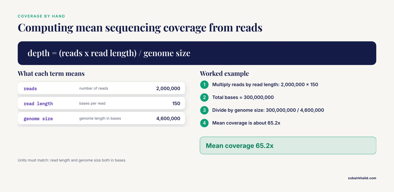
Suppose you sequence a bacterial genome of 4,600,000 bases and get 2,000,000 reads of 150 bases each.
reads = 2_000_000
read_length = 150
genome_size = 4_600_000

total_bases = reads * read_length
coverage = total_bases / genome_size
print(f"Total bases: {total_bases:,}")
print(f"Mean coverage: {coverage:.1f}x")
Expected output:
Total bases: 300,000,000
Mean coverage: 65.2x
Check the result by hand: 2 million times 150 is 300 million, and 300 million divided by 4.6 million is about 65. This single calculation is the foundation of depth-based quality decisions. Real genome reconstruction workflows treat coverage as a first-class quantity, flagging low-coverage regions and deletions as reliability problems rather than ignoring them 1. When a pipeline reports that part of a genome has shallow depth, that warning is this arithmetic made operational.
Step 2. Compute GC content and a log2 fold change
sequence = "ATGGCCTAAGGCATT"
gc = (sequence.count("G") + sequence.count("C")) / len(sequence)
print(f"GC content: {gc:.1%}")

control_mean = 100
treated_mean = 800
log2fc = np.log2(treated_mean / control_mean)
print(f"Log2 fold change: {log2fc:.2f}")
Expected output:
GC content: 42.9%
Log2 fold change: 3.00
The fold change is 8, and log2 of 8 is 3, meaning the gene is 2 to the power of 3 times higher in the treated sample. A log2 fold change of -2 means a quarter of the control level. Check the result by asking whether the sign and magnitude match the raw ratio. An 8-fold increase must give +3, never -3.
Step 3. Normalize counts with CPM and TPM
Raw counts are not comparable across samples because a sample with more total reads has higher counts for everything. Create a small count table and normalize it.
import pandas as pd

counts = pd.DataFrame(
    {
        "sample_1": [200, 50, 750],
        "sample_2": [400, 100, 1500],
    },
    index=["geneA", "geneB", "geneC"],
)

gene_lengths_kb = pd.Series([2.0, 5.0, 1.0], index=counts.index)

library_sizes = counts.sum()
cpm = counts.div(library_sizes, axis="columns") * 1_000_000

rpk = counts.div(gene_lengths_kb, axis="rows")
scaling = rpk.sum(axis="rows") / 1_000_000
tpm = rpk.div(scaling, axis="columns")

print(cpm.round(1))
print(tpm.round(1))
Expected output:
          sample_1  sample_2
geneA        166.7     166.7
geneB         41.7      41.7
geneC        625.0     625.0

          sample_1  sample_2
geneA       3030.3    3030.3
geneB        378.8     378.8
geneC       5681.8    5681.8
Sample 2 has exactly double the counts of sample 1, so after normalization the two samples agree, which is the whole point. Check the result two ways. First, CPM values within a sample should sum to exactly 1,000,000. Second, TPM values within a sample should also sum to 1,000,000. If either sum is off, the most common cause is dividing along the wrong axis.
The difference between the two measures matters in practice. CPM corrects only for library size, so a long gene tends to accumulate more reads and look more highly expressed. TPM divides by gene length first, which is why TPM is preferred when comparing the expression levels of different genes. Both are descriptive normalizations, and neither replaces the model-based normalization used in formal differential expression tools.
Step 4. Test for differences and correct for multiple testing
Build a tiny dataset with four genes measured in three control and three treated samples, run a t-test per gene, then apply Benjamini-Hochberg correction.
from scipy import stats
from statsmodels.stats.multitest import multipletests

data = pd.DataFrame(
    {
        "ctrl_1": [100, 200, 300, 105],
        "ctrl_2": [110, 190, 290, 95],
        "ctrl_3": [ 90, 210, 310, 100],
        "trt_1":  [800, 220, 320, 110],
        "trt_2":  [790, 180, 300,  90],
        "trt_3":  [810, 200, 340, 100],
    },
    index=["geneA", "geneB", "geneC", "geneD"],
)

control = data[["ctrl_1", "ctrl_2", "ctrl_3"]]
treated = data[["trt_1", "trt_2", "trt_3"]]

raw_p = []
for gene in data.index:
    t, p = stats.ttest_ind(treated.loc[gene], control.loc[gene])
    raw_p.append(p)

raw_p = np.array(raw_p)
reject, p_adj, _, _ = multipletests(raw_p, alpha=0.05, method="fdr_bh")

result = pd.DataFrame(
    {
        "raw_p": raw_p.round(5),
        "fdr_p": p_adj.round(5),
        "significant": reject,
    },
    index=data.index,
)
print(result)
Expected output:
         raw_p   fdr_p  significant
geneA  0.00003  0.00012         True
geneB  0.73666  0.73666        False
geneC  0.73666  0.73666        False
geneD  0.73666  0.73666        False
Gene A jumps from roughly 800 to roughly 100 between groups while the others barely move, so only gene A survives correction. Check the result by confirming that every adjusted p-value is greater than or equal to its raw p-value, which is always true for FDR correction. If you see adjusted values smaller than raw values, you passed the wrong array or the rows are out of order.
The Bonferroni alternative is one division. For a planned family of 20,000 tests at alpha 0.05, the per-test threshold is 0.05 divided by 20,000, which is 0.0000025. Bonferroni controls the chance of even one false positive and is correspondingly strict. Benjamini-Hochberg controls the expected proportion of false discoveries among the genes you call significant, which is usually the better fit for genome-scale screens.
Step 5. Compress a matrix with PCA
Principal component analysis rotates a genes-by-samples matrix so that the first axis captures the largest possible variance. Build a matrix where sample group drives most of the variation.
from sklearn.decomposition import PCA
from sklearn.[preprocessing](/blog/data-analysis/what-is-data-preprocessing) import StandardScaler

X = data.T.to_numpy()
X_scaled = StandardScaler().fit_transform(X)

pca = PCA(n_components=2)
scores = pca.fit_transform(X_scaled)

print("Explained variance ratio:",
      pca.explained_variance_ratio_.round(2))
print("Sample scores (rows are samples):")
print(scores.round(2))
Expected output, with exact decimals depending on your library version:
Explained variance ratio: [0.79 0.09]
Sample scores (rows are samples):
[[-3.05 -0.05]
 [-3.05  0.16]
 [-3.03 -0.11]
 [ 3.03 -0.05]
 [ 3.03  0.16]
 [ 3.05 -0.11]]
The three control samples land at strongly negative values on the first component and the three treated samples at strongly positive values, so the treatment effect dominates, as the large explained variance ratio confirms. In real analyses this plot is the first place batch effects reveal themselves, and that diagnostic habit matters, because data integration methods in computational biology were developed precisely because batch effects and data complexity interfere with joint analysis of datasets from different sources 5. Representation learning methods for single-cell data target the same problem, learning low-dimensional representations that remove batch effects while keeping cell type structure intact 6.
Check the result by re-plotting with matplotlib and asking a biological question: do the samples separate by the variable you care about, or by something you did not plan, such as processing date? A separation you did not design is a finding to investigate, not decoration.
Step 6. Diagnose the errors you will actually hit
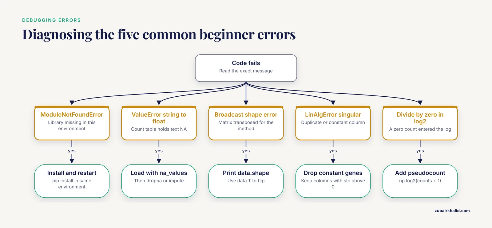
These are the five error messages beginners encounter most, with the exact text and the fix.
ModuleNotFoundError: No module named 'statsmodels'. The library is not installed in the environment your notebook is using. Run python -m pip install statsmodels in the same environment, or restart the kernel after installing.
ValueError: could not convert string to float: 'NA'. Your count table contains missing values written as text. Load the table with pd.read_csv("counts.csv", na_values=["NA"]) and then either drop incomplete rows with data.dropna() or impute them, and state which you did.
ValueError: operands could not be broadcast together with shapes (6,4) (4,6). Your matrix is transposed relative to what the operation expects. Print data.shape and confirm that rows are samples where the method expects them. data.T flips the orientation.
LinAlgError: Singular matrix. One of your columns is a perfect duplicate or constant, so the matrix cannot be inverted. Remove constant genes with data.loc[:, data.std() > 0] before fitting.
RuntimeWarning: divide by zero encountered in log2. A count of zero went into a logarithm. Add a pseudocount, for example np.log2(counts + 1), which is standard practice, and mention it in your methods.
How These Skills Show Up in Real Pipelines
Seeing the math embedded in published work is the fastest cure for the feeling that it is abstract homework. The examples below each use one or two items from the inventory.
Genome reconstruction pipelines for SARS-CoV-2 from amplicon sequencing depend on coverage arithmetic, allele fraction thresholds for detecting mixed samples, and judgment about low-coverage regions near primer sites, where lineage-determining mutations can hide 1. A person who cannot compute mean coverage or interpret an allele fraction near 0.5 cannot debug such a pipeline, and a person who can, can.
Viral genomics for therapeutic phage development leans on genome quality assessment, gene prediction and annotation, lifestyle classification, and host prediction, each of which outputs scores and probabilities that require statistical literacy to interpret and validate 7. Reading a tool's output table, knowing what a classification probability means, and knowing when to distrust it is applied math.
Discriminant analysis methods such as PANDA formulate their objective directly in the language of between-class and within-class variance, then learn shared representations across omics types so that correlation and discrimination do not have to be traded off against each other 3. If you understand variance and covariance, the method's core idea fits in one sentence.
Machine learning in clinical microbiology is described in the literature as a lifecycle with defined stages: problem definition, data preparation, feature engineering, hyperparameter optimization, and evaluation, with specific attention to class imbalance, generalization, and interpretability 8. Every one of those stages has a small mathematical core, and the lifecycle framing tells you which math to learn at which stage.
Ensemble prediction of enhancer-promoter loops integrates several omics feature types with modest input requirements, showing that well-chosen features often beat exotic mathematics 9. Gene shaving work in cancer data illustrates the evaluation habit you should copy: performance was reported as true positive rate, false discovery rate, and area under the curve, on both simulated and real data, and the method identified 210 candidate genes out of 2,000 in a colon cancer dataset 2.
High-dimensional outcome modeling in radiomics and radiogenomics explicitly warns about the central statistical danger of many features and few patients, and discusses harmonization strategies for combining data across centers 10. Genomic selection in polyploid crops such as banana highlights dominance, epistasis, and genotype-by-environment interaction as modeling challenges that diploid-oriented tools handle poorly 11. Serological biomarker work for malaria exposure fits antibody decay curves to estimate the timing and intensity of past infection, a direct application of regression to public health surveillance 12.
Two more examples round out the picture. A cross-staining deep learning study in breast histopathology reported recognition accuracy of 89.6 percent on H&E-stained images and 80.5 percent on fluorescent-stained images, and the gap between those numbers is itself a lesson in how preprocessing choices, here color normalization, move evaluation metrics 4. At the workflow level, tools for federated learning are embedded in reproducible Snakemake pipelines and compared against centralized analyses, which is a reminder that orchestration and reproducibility, not exotic mathematics, are what make multi-site computational science trustworthy 13. And integrative transcriptomic studies that combine differential expression, network analysis, enrichment, molecular docking, and molecular dynamics simulation, in one neurological disease study running 500-nanosecond simulations, show how the math scales upward once the foundations are in place 14.
The pattern across all of it: the mathematics is layered, and each layer is small.
How to Overcome Math Anxiety in Bioinformatics
Math anxiety is a learned stress response to perceived evaluation, not a fixed ability limit, and it responds to the same things any fear responds to: graded exposure, quick wins, and evidence that contradicts the feared belief. Here are the bioinformatics math requirements tips that consistently work, drawn from how working analysts actually learn.
Learn math on demand, anchored to a real dataset. Anxiety thrives on abstraction. A person who sits down to "learn statistics" faces an unbounded task. A person who sits down to find genes that differ between two conditions faces a bounded task, and the statistics arrives as the tool for that task. Download a small public dataset, pick one biological question, and let the question pull each math topic in exactly when needed. This is the single highest-yield change you can make to how you learn bioinformatics.
Practice in 20-minute daily blocks, not weekend marathons. Procedural skills, including arithmetic with scientific notation and reading log scales, consolidate with spaced repetition. Twenty focused minutes per day for a month beats an eight-hour crash that leaves you drained and reinforces the association between math and misery.
Keep an error journal. Every time code fails, write the exact error message and the fix in one file. Within a month you will have a personal reference of the ten errors that account for most failures, including the ones listed in Step 6 above. Rereading that file produces a concrete, visible record of competence, which directly counters the anxious belief that you are always confused.
Verify one calculation by hand, then automate it. Do the CPM arithmetic for one gene with a calculator, then let pandas do it for 30,000 genes. The hand calculation converts the formula from a black box into something you own, and owning even one formula per concept measurably lowers the threat level of the rest.
Turn physical symptoms into a signal to slow down, not a signal to stop. Racing heart and tunnel vision before opening a statistics chapter are arousal, not evidence of inability. Naming the state and proceeding slowly, with easier material first, reliably reduces the response over weeks.
Work with people. A weekly one-hour session with one other learner, where you each explain one concept aloud, outperforms solo study for retention and for anxiety, because explaining forces the reorganization that passive reading never triggers. Bioinformatics communities on forum platforms and in course cohorts exist precisely for this.
Build plots before derivations. Plot a histogram of p-values from your own analysis. Plot raw counts against library size and watch the trend that motivates normalization. Visualization converts an abstract rule into a picture you can recall under stress, and pictures are more anxiety-resistant than formulas.
Track progress in a visible place. A dated list of concepts you have used successfully, with the project they appeared in, gives you a document to consult on bad days. Anxiety compresses memory for successes and expands memory for failures, and the list corrects the imbalance.
If anxiety is severe enough to block study entirely, campus counseling services and licensed therapists treat it effectively, and there is no downside to starting there alongside the practices above.
Choosing and Using a Bioinformatics Course
A bioinformatics course accelerates all of the above if you pick it with the math inventory in mind. Use these criteria.
Choose project-based over lecture-complete. The best courses make you compute coverage, normalize a count table, run a test, correct for multiple comparisons, and interpret a PCA plot on real data within the first weeks. Courses that front-load months of pure mathematics before any data tend to feed anxiety rather than fix it.
Check that the course teaches decisions, not just commands. Running a tool is easy. Knowing why a workflow clips primers before variant calling, or why low-coverage regions are flagged rather than silently accepted, requires the conceptual layer, and published pipeline papers are explicit that these decision points are where analyses succeed or fail 1.
Demand reproducibility habits from week one. A course that has you write a Snakemake or Nextflow workflow, or even a clean notebook with fixed seeds and recorded versions, teaches the professional standard. Reproducible workflow tooling is now a mainstream expectation in published bioinformatics, including for multi-institution and federated analyses 13.
Match the course to your domain. Microbiologists benefit from courses framed around the ML lifecycle and clinical evaluation 8. Breeders and population geneticists benefit from quantitative genetics framing(https://pubmed.ncbi.nlm.nih.gov/36388523/). A general course is fine to start, but your second course should speak your data's language.
Sequence your math alongside the course, not before it. Weeks 1 to 2, arithmetic, logs, and normalization. Weeks 3 to 4, descriptive statistics and hypothesis testing. Weeks 5 to 8, multiple comparisons and PCA. Months 3 and beyond, linear algebra depth, Bayesian thinking, and the calculus fragments behind optimization. This ordering matches how the skills appear in the literature you will eventually read.
Common Mistakes and Limitations
These are the errors that cost beginners the most time, stated plainly.
Front-loading all the math before touching data. Waiting until you "finish" mathematics before starting bioinformatics is the most common self-imposed blocker, and it is unnecessary. Every topic in the inventory can be learned in the context of an analysis, and context is what makes it stick.
Taking log2 of zero without a pseudocount. The result is negative infinity, which then poisons every downstream mean and test. Add 1 to counts before logging, consistently, everywhere.
Comparing raw counts across samples. A gene with 500 reads in a 30-million-read sample is less abundant than a gene with 400 reads in a 5-million-read sample. Normalize first, always, and know which normalization you used.
Treating FDR-adjusted values as ordinary p-values. An FDR-adjusted value of 0.05 means that about 5 percent of the discoveries in your list are expected to be false, not that this single test had a 5 percent chance of a false positive under a true null. The distinction changes how you describe results in a paper.
Reporting significance without effect size. With 20,000 tests, tiny fold changes can be significant. Report the log2 fold change next to the adjusted p-value, and filter or rank on both.
Ignoring batch effects and scale differences. Datasets from different labs, platforms, and batches carry technical variation that mixes with biology, which is the central problem that data integration research addresses 5, and single-cell integration methods exist because naive merging destroys biological signal 6. Before combining datasets, plot them and look for structure that tracks with batch rather than biology.
Fitting complex models to small samples. High-dimensional prediction with few observations invites overfitting, a warning that recurs across radiomic modeling 10 and that motivates validation gates in translational genomics reviews 7. Hold out data. Report performance on the held-out data. Be suspicious of models that look perfect on training data.
Skipping the assumptions of your test. A t-test on raw, heavily skewed counts is often the wrong tool, and transformations or non-parametric alternatives exist for a reason. Check the distribution with a plot before you test.
Confusing a prediction with an explanation. A model can rank samples well and still tell you nothing about mechanism, and interpretation is a distinct, explicit stage in rigorous ML practice 8.
One limitation deserves its own sentence. For decisions that carry clinical, regulatory, or publication stakes, an experienced statistician or analyst should review the analysis plan before data are locked, because no self-teaching path substitutes for that review.
Frequently Asked Questions
Do I need calculus for bioinformatics?
No, not for most work. You need the concept of a slope to understand how models are optimized, but day-to-day tasks in genomics and pipelines use arithmetic, logarithms, and statistics rather than calculus.
How much statistics do I need to learn bioinformatics?
Enough to compute and interpret means, variance, a t-test, p-values, and multiple testing correction, which is roughly one introductory statistics course worth of material, learnable in weeks when anchored to real data.
Can I learn bioinformatics if I am bad at math?
Yes. Math anxiety reflects practice history, not ability, and the mathematics bioinformatics actually requires is a narrow, learnable set that responds quickly to daily short practice sessions on real datasets.
What math do I need for machine learning in bioinformatics?
Linear algebra for matrices, descriptive statistics, classification and evaluation metrics, and the concept of optimization, with the ML lifecycle stages of data preparation, model development, and evaluation as your learning map.
How long does it take to learn the math for bioinformatics?
Four to eight weeks of daily 20-minute practice covers the core inventory well enough to run and interpret a complete small analysis, with deeper statistics and linear algebra accumulating over subsequent months.
Is linear algebra really necessary for omics data?
A working understanding is necessary, because expression matrices, PCA, and integration methods are all matrix operations, but derivation-level depth is not required to apply and interpret the methods correctly.
How do I overcome math anxiety while learning bioinformatics?
Use graded exposure with quick wins: learn each topic on demand inside a real project, practice daily in short blocks, keep an error journal as visible proof of progress, and verify one calculation by hand before automating it.
Do I need math to run existing bioinformatics pipelines?
You can run a finished pipeline with almost none, but interpreting its quality control numbers, coverage warnings, and statistical outputs requires the inventory in this article, and interpretation is the part that matters.
Sources
- Lessons learned: overcoming common challenges in reconstructing the SARS-CoV-2 genome from short-read sequencing data via CoVpipe2.
- Gene shaving using a sensitivity analysis of kernel based machine learning approach, with applications to cancer data.
- Joint multi-omics discriminant analysis with consistent representation learning using PANDA.
- Deep-learning based breast cancer detection for cross-staining histopathology images.
- Omics data integration in computational biology viewed through the prism of machine learning paradigms.
- Integration of single cell data by disentangled representation learning.
- Phage Genomics and Bioinformatics in Therapeutic Development: Evidence Limits, Validation Gates, and Translational Decision-Making.
- An introduction to the machine learning lifecycle for clinical microbiology.
- Predicting unrecognized enhancer-mediated genome topology by an ensemble machine learning model.
- Radiomic and radiogenomic modeling for radiotherapy: strategies, pitfalls, and challenges.
- Perspective for genomic-enabled prediction against black sigatoka disease and drought stress in polyploid species.
- Novel bioinformatic methods and machine learning approaches reveal candidate biomarkers of the intensity and timing of past exposure to Plasmodium falciparum.
- Fedflow: cloud orchestration for federated learning with the FeatureCloud platform.
- Integrative Transcriptomic and Network Analyses Reveal Common Molecular Signatures and Turmeric-Derived Common Therapeutic Candidates for Neurological Diseases.