Bioinformatics Core Concepts: Complete Guide
By Dr. Zubair Khalid, DVM, MS, PhD ·
Bioinformatics is the discipline that applies computing, statistics, and information technology to biological data, most often data derived from DNA, RNA, proteins, and other molecular measurements. Bioinformatics core concepts are the shared foundation under every analysis: how biological data is produced and stored, how sequences are compared, how statistical claims are made from noisy measurements, and how results are kept trustworthy and reproducible.
These concepts matter because modern biology has become a data science. A single sequencing run can generate hundreds of gigabytes of raw reads, and a single study may combine genomes, transcriptomes, clinical records, and imaging. Without the core concepts, that data is unreadable noise. With them, researchers can trace a drug resistance mutation across hundreds of bacterial genomes [1], build diagnostic pipelines that take sequencing data from raw fragments to clinically actionable biomarkers [2], and design multi-scale models of disease that connect molecules to tissues [3]. Whether your goal is to learn bioinformatics for a degree, a career change, or a single project, every practical skill builds on the same small set of ideas explained below.
What Are Bioinformatics Core Concepts? (Bioinformatics Core Concepts Explained)
Students asking "what is bioinformatics core concepts" usually want a list they can hang skills on. The consensus of standard textbooks and professional training programs organizes the field around seven concepts:
- Biological data and its formats, including raw sequence reads, reference genomes, and annotation files
- Sequence alignment, the comparison of sequences to find similarity and infer relatedness
- Assembly and reference mapping, turning reads into genomes or positioning reads on a known genome
- Annotation and databases, attaching biological meaning (genes, functions, pathways) to raw sequence
- Statistical inference, deciding whether a measured difference is real or sampling noise
- Machine learning and AI, building predictive models from biological data
- Reproducibility and data management, making analyses documented, portable, and shareable
Each concept is a layer. The first four deal with turning raw signal into biological objects. The fifth and sixth deal with turning biological objects into claims. The last deals with making all of it trustworthy. A person who understands these seven layers can read almost any genomics paper, follow almost any bioinformatics course syllabus, and learn new tools quickly because new tools almost always slot into one of these layers.
Bioinformatics and Its Neighboring Fields
Bioinformatics is often confused with computational biology, biostatistics, and data science. The terms overlap but describe different centers of gravity, and knowing the difference helps you pick the right training and vocabulary.
| Term | Center of gravity | Typical question | Typical output |
|---|---|---|---|
| , - | , - | , - | , - |
| Bioinformatics | Data processing pipelines for biological data | How do I turn these raw reads into a count matrix or genome assembly? | Scripts, pipelines, annotations |
| Computational biology | Models of biological systems | How do these molecules behave as a system over time? | Mechanistic or predictive models |
| Biostatistics | Inference from experimental design | Is this treatment effect statistically supported? | Confidence intervals, p values, power calculations |
| Data science / ML | Prediction from learned patterns | Can I predict resistance or outcome from these features? | Trained models with validated performance |
In practice one person often works across several columns. A study of antimicrobial resistance, for example, may need pipeline work to process bacterial genomes, statistical work for a genome-wide association study, machine learning for prediction, and wet-lab work for validation [1]. The labels describe emphases, not walls.
Core Concept 1: Biological Data and Its Formats
Everything in bioinformatics starts with data produced by laboratory instruments, and the first core skill is knowing what those instruments measure and how that measurement is encoded.
Where the data comes from
The dominant technology is next-generation sequencing (NGS), a family of methods that reads DNA or RNA by sequencing millions to billions of short fragments in parallel. NGS underpins whole-genome sequencing, RNA sequencing (RNA-seq) for measuring gene expression, and small RNA sequencing for measuring microRNAs (miRNAs), the short regulatory RNAs now studied as cancer biomarkers [2]. Other omics layers include proteomics (proteins measured mostly by mass spectrometry), metabolomics (small molecules), and the exposome, the sum of all environmental exposures a person encounters from conception to death, which spans chemical exposures, diet, and social factors [4].
How sequence data is encoded
The workhorse file formats are worth memorizing because they appear in every workflow:
- FASTA stores one or more sequences. Each record starts with a header line beginning with
>followed by the sequence itself, either DNA, RNA, or protein in single-letter codes. - FASTQ stores sequence plus per-base quality scores from a sequencer. A record has four lines: a header starting with
@, the sequence, a+line, and a quality string where each character encodes a Phred score. - SAM and BAM store aligned reads. SAM is text, BAM is its compressed binary equivalent. Tools such as samtools read and manipulate them.
- VCF (Variant Call Format) stores genetic differences, called variants, between a sample and a reference genome.
- GTF/GFF store genome annotation, mapping coordinates to genes, transcripts, and exons.
The Phred quality score is the standard quality metric. It is defined as Q = -10 log10(P), where P is the probability the base call is wrong. A Phred score of 20 means a 1 in 100 chance of error, and a score of 30 means a 1 in 1,000 chance of error. Quality profiles decline toward the ends of reads, which is why read trimming and quality filtering appear near the start of nearly every pipeline.
A minimal FASTQ record looks like this:
@read_0001
GATCGATTGCAGTCAG
+
IIIIIHHHHHF#5FII
The quality characters on the fourth line are ASCII-encoded scores. Low scores such as # mark bases likely to be wrong.
Core Concept 2: Sequence Alignment
Alignment answers the most common question in sequence analysis: how similar are these two sequences, and where do they match? Similarity is the evidence behind inferring shared ancestry, transferred function, and the presence of genes or variants.
Pairwise alignment and scoring
Pairwise alignment arranges two sequences, allowing gaps, to maximize a score. Two classic algorithms define the field. The Needleman-Wunsch algorithm performs global alignment, aligning sequences end to end. The Smith-Waterman algorithm performs local alignment, finding the best matching segment within longer sequences. Both are dynamic programming methods that score matches, mismatches, and gaps.
Scores depend on a substitution matrix, most commonly BLOSUM62 for proteins, which rewards conservative amino acid substitutions and penalizes unlikely ones. Gap penalties, usually a larger cost to open a gap and a smaller cost to extend it, prevent alignments from shattering into trivial fragments.
Heuristic database search
Comparing a query against millions of database sequences with full dynamic programming is too slow, so database search tools use heuristics. BLAST (Basic Local Alignment Search Tool) finds short exact or near-exact seed matches and extends them, reporting hits with an E-value, the expected number of random matches of that score in a database of that size. A low E-value, such as 1e-50, means the match is extremely unlikely to occur by chance. The BLAST E-value, not the raw percent identity, is the number that tells you whether a hit is meaningful.
Aligning millions of short reads
For resequencing, where millions of short reads are placed onto a reference genome, alignment relies on compressed index structures built with the Burrows-Wheeler Transform (BWT). Tools in this family, such as BWA and Bowtie, align reads orders of magnitude faster than exhaustive search by trading a small amount of sensitivity for enormous speed. A typical mapping step reports a mapping rate, the percentage of reads placed on the reference, which serves as a first quality check on the entire experiment.
Core Concept 3: Assembly, Reference Mapping, and Variant Calling
Raw reads are fragments. Two strategies reconstruct biology from them.
De novo assembly versus reference-based analysis
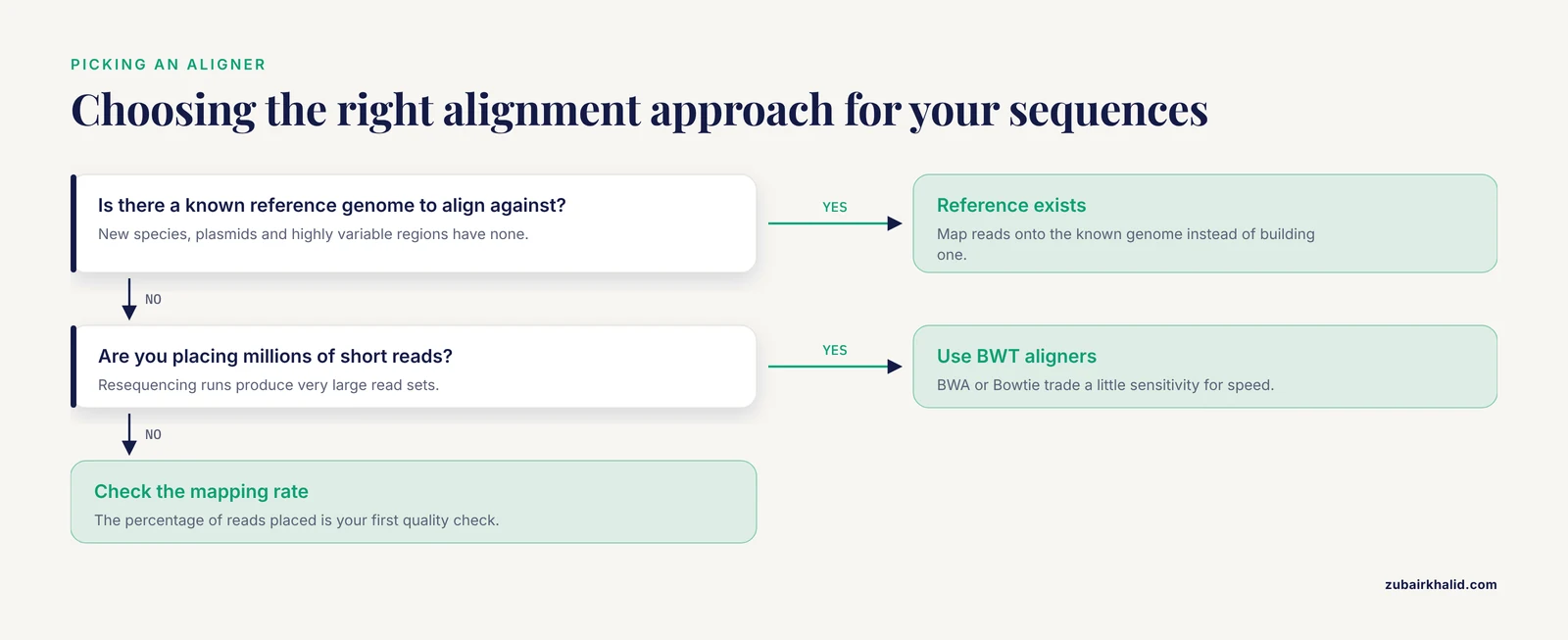
De novo assembly builds a genome from reads alone, with no reference. Assemblers break reads into overlapping pieces and resolve them into contigs and scaffolds. This approach is required for new species, plasmids, and regions too variable to align.
Reference mapping aligns reads to an already sequenced genome. This is faster and simpler and is the default for human clinical and research sequencing. Once reads are mapped, the pileup of bases at each position lets a variant caller distinguish true differences from sequencing errors. Variant calling produces the VCF files that feed association studies, such as the genome-wide association studies (GWAS) used to find resistance mutations in bacterial collections [1].
Coverage
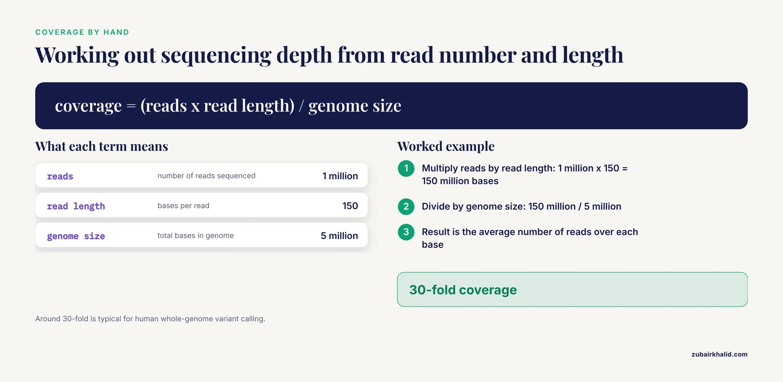
Coverage (or depth) is the average number of reads overlapping each base. It is calculated as the product of read number and read length divided by genome size. A 150-base read giving 30-fold coverage of a 5 million base genome means 1 million reads were sequenced. Low coverage leaves gaps and errors, while extremely high coverage wastes budget, so depth planning is a design decision, not an afterthought. Standard textbook practice treats around 30-fold coverage as typical for human whole-genome variant calling, with deeper coverage for applications such as RNA-seq heterogeneity or somatic mutation detection in tumors.
Core Concept 4: Annotation and Databases
A sequence string has no meaning until it is annotated. Annotation attaches names, functions, pathways, and structure to sequence coordinates, and it depends on curated public databases.
What annotation does
Gene prediction identifies coding regions. Functional annotation transfers information from known genes to new sequences by similarity, for example labeling a predicted protein as a kinase because it matches known kinase domains. Pathway annotation maps genes onto metabolic and signaling pathways so that a list of differentially expressed genes can be interpreted as a coherent biological process. In the miRNA field, annotation and pathway analysis tools such as DIANA-miRPath link measured microRNAs to the biological pathways their targets affect, a step the current literature treats as part of an integrated analysis pipeline rather than an afterthought [2].
Databases as shared infrastructure
Curated public databases act as the field's shared memory. Sequence archives store raw reads, reference genomes provide the coordinate systems, and protein databases such as UniProt provide curated functional information. The guiding principle, emphasized across reviews of data-intensive biology, is that data must be described with precise ontologies and standardized vocabulary before it can be integrated into high-value datasets [5]. An ontology is a controlled, structured vocabulary in which terms have defined relationships, so that "drug resistance" means the same thing in every dataset that uses the term.
Core Concept 5: Statistical Inference in Bioinformatics
Biology is noisy, and the biggest conceptual jump for new students is learning that bioinformatics is as much statistics as it is computing.
From counts to calls
Most omics experiments compare groups, for example tumor versus normal tissue. The measured quantity is a count or an intensity, and the question is whether the difference between groups exceeds what sampling variation would produce. RNA-seq differential expression tools such as DESeq2 and edgeR model counts with negative binomial distributions, estimate dispersion, and test each gene with a null hypothesis of no difference.
The multiple testing problem
Testing 20,000 genes at a conventional p value threshold of 0.05 produces about 1,000 false positives by chance alone. The standard solution is false discovery rate (FDR) control, most often the Benjamini-Hochberg procedure, which adjusts thresholds so that, among the genes you call significant, a controlled fraction are expected to be false discoveries. Reporting an FDR-adjusted p value (a q value) rather than a raw p value is one of the clearest markers that an analysis was done competently.
Association analysis
Association testing extends inference to genotype. In a GWAS, millions of variants are tested for correlation with a trait, and stringent genome-wide thresholds plus corrections for population structure are required to avoid false signals. A published example in Streptococcus pneumoniae used GWAS across 662 clinical genomes to identify variants associated with trimethoprim resistance, then confirmed the finding biologically rather than statistically alone [1]. The association step is one layer of evidence, never the whole argument.
Core Concept 6: Machine Learning and AI in Bioinformatics
Machine learning (ML) builds predictive models from data instead of testing predefined hypotheses. It is now embedded in nearly every area of computational biology, and the literature describes a coherent progression from classical ML to deep learning to large language models.
The standard learning framework
Supervised learning trains a model on labeled examples, for example genomes labeled resistant or susceptible, to predict labels for new samples. Common algorithms include support vector machines (SVMs), random forests, and gradient boosting. Unsupervised learning, such as principal component analysis and clustering, finds structure without labels and is often used for quality control, batch detection, and sample grouping. Model development requires disciplined splitting of data into training and test sets, transparent and reproducible data processing, careful choice of data representation, and honest estimates of prediction uncertainty [5]. Models evaluated on the same data they were trained on are inflated and useless.
Deep learning and language models
Deep learning (DL) uses layered neural networks that learn their own feature representations. Convolutional neural networks (CNNs) excel at spatial patterns such as sequence motifs and images, and recurrent neural networks (RNNs) handle sequential data such as nucleotide and amino acid chains. Reviews of miRNA bioinformatics describe this exact progression, from pipeline tools such as miRDeep2 for discovering microRNAs from NGS data, through SVM, CNN, and RNN layers for signature identification and target prediction, to generative models and large language models (LLMs) that support hypothesis generation and reproducibility in biomarker discovery [2].
Machine learning with validation, not instead of validation
The strongest recent work pairs ML with experimental confirmation. In the S. pneumoniae trimethoprim study, GWAS identified candidate resistance mutations in the folA and sulA loci, resistance reconstruction experiments in the laboratory validated those mutations functionally, and ML models predicting minimum inhibitory concentration (MIC), the lowest antibiotic concentration that inhibits growth, reached an average accuracy within plus or minus one twofold dilution of the observed MIC in 86.3% of cases [1]. The published roadmap, moving from in silico analysis to wet-lab validation to diagnostic tool building, is a template worth internalizing because it treats prediction as a hypothesis generator, not a final answer.
A separate, less glamorous ML application is knowledge synthesis. Literature-based ML classifiers can semiautomate systematic reviews, for example training models to classify and extract data from PubMed records at the intersection of liver cancer, epidemiology, and health disparities research. One such six-phase workflow, covering training, validation, confirmation, error analysis, extraction model development, and application, achieved high classifier accuracy with limited training data, reporting standard metrics of precision, recall, F1, and accuracy at each phase [6]. This shows students that bioinformatics ML is not only sequence prediction. It also includes extracting structure from text, a task increasingly shared with LLMs.
Core Concept 7: Systems Biology and Multi-Scale Modeling
Sequence-level analysis treats parts in isolation. Systems biology asks how the parts behave together, modeling cancer, infection, or metabolism as networks of interacting molecules, cells, and tissues [3]. Models in this tradition range from differential equation models of signaling pathways to agent-based models of tumor growth and constraint-based models of microbial metabolism.
A 2025 roadmap from the cancer systems biology community argues that the field's central promise, predicting how specific molecular changes produce altered disease outcomes, remains incompletely fulfilled, and that progress depends on better coordination between modeling groups and data-generating groups so that multiscale models can be built on consistently structured data [3]. For a student, the practical lesson is that pipelines and models are not separate career tracks. Data producers, pipeline builders, and modelers depend on each other, and the interface between them, agreed data formats and metadata standards, is where much of the real work happens.
Core Concept 8: Reproducibility, Data Governance, and Sharing
The final core concept is the one that separates a demo from a scientific result. A bioinformatics result exists only if someone else can rerun it and get the same answer, and only if the underlying data was handled legally and ethically.
Technical reproducibility
Practical reproducibility rests on standard infrastructure that any bioinformatics course should teach:
- Workflow managers such as Snakemake and Nextflow encode every step, parameter, and dependency in a script so the entire analysis reruns with one command.
- Environment management with conda or containers such as Docker and Apptainer pins software versions, because a result produced with tool version X is not guaranteed to match one produced with version Y.
- Version control with Git records every change to code.
- Public repositories for raw data and code let reviewers and readers audit the work from raw reads to figures.
Reviews of data-intensive research consistently emphasize transparent, reproducible data processing as a prerequisite for trustworthy machine learning, alongside well-defined training and test sets and quantified prediction uncertainty [5].
Data governance and sharing across jurisdictions
Sharing human data raises obligations that pure code does not. An expert consultation spanning child health, genomics, bioethics, privacy, and law identified recurring barriers to sharing pediatric research data across borders, including a lack of standardized consent, complicated ethics review for multi-site projects, the need for data governance frameworks aligned with institutional and regulatory requirements, and differing data standards between centers [7]. A large international pediatric arthritis network that collects and shares phenotypic, genomic, and patient-reported data across Canada and the Netherlands was documented specifically as a practical, real-life example of solving these barriers [7].
When data cannot legally move, data federation is the emerging alternative. In federation, data stays at its source institution and analyses travel to the data, an approach proposed for the exposomics community precisely because exposure data is scattered across many resources with varying privacy, access, and analysis constraints [4]. Students should understand both models, centralized sharing and federated query, because real projects rarely get to choose freely.
A Worked Example: One Study, All the Core Concepts
Tracing a single published study through the concepts shows how they interlock in practice. The trimethoprim resistance study in Streptococcus pneumoniae [1] runs as follows:
- Data production. NGS produced whole-genome sequences for 662 clinical isolates, each with an MIC measurement for trimethoprim susceptibility.
- Processing. Reads were mapped to a reference, variants were called, and genomes were encoded as variant matrices, applying concepts 1 through 3.
- Association. A GWAS tested variants against resistance phenotype, implicating additive mutations in the folA and sulA loci, applying concept 5.
- Functional validation. Resistance reconstruction experiments transferred candidate mutations into laboratory strains and confirmed their effects, adding biological evidence beyond statistics.
- Machine learning. The validated mutations served as features for ML models that predicted MIC digitally, reaching 86.3% accuracy within one twofold dilution, applying concept 6.
- Translation. The authors framed the result as a reusable roadmap from computational analysis to laboratory validation to diagnostic development, applying concept 7's systems view and concept 8's emphasis on shareable, standardized outputs [1].
This is what "bioinformatics core concepts explained" looks like in a real paper. No single step is exotic. The value comes from connecting them correctly.
How These Concepts Are Learned and Tested in Practice
If your goal is to learn bioinformatics, the concepts above translate into a concrete skill ladder that most graduate courses and professional training programs follow.
The practical skill ladder
- Command line fundamentals. File manipulation, text processing, and shell scripting. Most bioinformatics tools are command line programs, so this comes first.
- One scripting language deeply. Python and R dominate. R with Bioconductor is standard for statistical genomics, Python for pipelines, ML, and general tooling.
- Core file formats and tools. Reading and manipulating FASTA, FASTQ, SAM/BAM, VCF, and GTF files with standard tools.
- One complete pipeline end to end. For example, taking an RNA-seq dataset from FASTQ files through quality control, alignment, quantification, differential expression, and pathway analysis.
- Statistics. Hypothesis testing, FDR correction, linear models, and experimental design.
- Reproducible workflows. Conda environments, Snakemake or Nextflow, Git, and containers.
- ML fundamentals. Cross-validation, train and test splits, feature selection, and performance metrics such as precision, recall, F1, and accuracy [6].
How competence is assessed
Assessment in courses and in hiring looks for the same things. You will be asked to debug a failing pipeline, interpret an alignment rate or a quality report, explain why an FDR threshold was applied, spot a machine learning evaluation that leaked test data into training, and reproduce a result from someone else's script. Benchmarking exercises, where different algorithms for the same task such as miRNA discovery are compared on shared datasets, are also part of the professional literature and a good way to build judgment [2].
Choosing a bioinformatics course
A strong bioinformatics course, whether a university semester, an EMBL-EBI or NCBI workshop, or a self-paced online program, shares three features. It teaches concepts before tools, gives hands-on access to real datasets rather than toy examples, and requires a complete reproducible project as the final output. Courses that only teach point-and-click web tools without the underlying formats and statistics leave students unable to debug anything. Courses that teach tools without biology leave students unable to interpret results. Aim for both.
Common Mistakes and Limitations
Every experienced analyst has made these errors. Knowing them in advance saves months.
- Treating percent identity as meaning. Two sequences can share 70% identity by chance. The E-value and the alignment length, not the identity percentage, determine whether a database hit means anything.
- Ignoring batch effects. Samples processed on different days, by different operators, or in different lanes carry systematic differences that can mimic biology. Unsupervised methods such as principal component analysis should be run before any differential analysis to check that samples group by biology, not by batch.
- Testing everything at a raw p value threshold. Testing thousands of features without FDR correction produces mostly false positives. This single error invalidates more amateur analyses than any other.
- Evaluating machine learning models on training data. A model that scores 99% on the data it memorized may score at chance on new data. Cross-validation and held-out test sets are mandatory, and prediction uncertainty should be reported, not hidden [5].
- Confusing correlation with mechanism. A GWAS hit is an association until an experiment, such as resistance reconstruction in a defined strain background, shows the variant actually causes the phenotype [1]. Data-driven methods find patterns, and patterns require biological validation.
- Skipping version pinning. Rerunning a pipeline with updated tool versions can change results. Environment files and containers exist for a reason.
- Underestimating data governance. Human genomic data usually cannot be uploaded to a public server. Consent terms, institutional review requirements, and jurisdictional privacy law constrain sharing, and these constraints need to be planned into a project from the beginning, not discovered at submission time [7].
- Assuming integration is free. Combining omics layers, clinical data, and exposure data requires ontologies, standardized vocabularies, and compatible formats. Data integration is a design problem, and reviews across drug discovery and exposomics converge on the same recommendation, invest in data structure early [5][4].
- A general limitation. Bioinformatics outputs are hypotheses and decision supports, not clinical diagnoses on their own. Individual cases, whether in medicine, microbiology, or agriculture, require confirmation by qualified professionals using validated laboratory and clinical methods.
Quick Review
- Bioinformatics applies computing and statistics to biological data, and its core concepts form the layers every analysis shares: data formats, alignment, assembly, annotation, statistics, machine learning, and reproducibility [1].
- FASTQ records sequence plus Phred quality, where Q30 means a 1 in 1,000 chance of a wrong base. Quality control comes before everything else.
- Alignment is scored with substitution matrices and gap penalties. BLAST hits are judged by E-value, and high-throughput read mapping uses BWT-based aligners such as BWA and Bowtie.
- The multiple testing problem is solved with false discovery rate control. Adjusted p values, not raw p values, are the standard for omics.
- Machine learning in bioinformatics spans SVMs, CNNs, RNNs, and LLMs, and trustworthy models require clean train and test separation plus quantified uncertainty [2][5].
- The strongest studies pair computational findings with experimental validation, as in the S. pneumoniae work where GWAS, resistance reconstruction, and ML produced a digital MIC predictor accurate to within one twofold dilution in 86.3% of cases [1].
- Reproducibility and governance are core concepts, not afterthoughts. Workflows, containers, and version control make results rerunnable, while consent, regulation, and data standards determine what can be shared at all [7][5].
Frequently Asked Questions
What are bioinformatics core concepts?
They are the foundational ideas every bioinformatics analysis rests on: biological data formats, sequence alignment, assembly and mapping, annotation and databases, statistical inference, machine learning, and reproducible data management. Mastering these seven areas lets you learn any new tool quickly, because new tools almost always fit into one of these layers.
Do I need to know programming to learn bioinformatics?
Yes, at least one language at a working level. Python and R are the standard choices, and comfort with the Unix command line is essential because most bioinformatics tools run there. You do not need to be a software engineer. You need to write, debug, and adapt scripts confidently.
What is the difference between bioinformatics and computational biology?
Bioinformatics centers on building and running pipelines that process biological data, such as turning raw sequencing reads into variant lists. Computational biology centers on building models of biological systems, such as simulating how a signaling network responds to a drug. The fields overlap heavily and many people work in both.
What is a concrete example of bioinformatics core concepts in action?
A study of antibiotic resistance in Streptococcus pneumoniae processed whole-genome sequences from 662 isolates, used GWAS to find resistance-associated mutations, validated them experimentally, and built a machine learning model that predicted antibiotic susceptibility with 86.3% accuracy within one twofold dilution [1]. Every stage of that study corresponds to one of the core concepts described above.
How do machine learning and AI fit into modern bioinformatics?
Machine learning adds predictive layers on top of standard pipelines, from support vector machines for classification to deep learning models such as CNNs and RNNs for sequence data, and large language models for literature synthesis and hypothesis generation. Reviews of miRNA-based cancer biomarker discovery describe an integrated framework that spans NGS processing, ML, and LLM support for reproducible biomarker workflows [2].
What should a good bioinformatics course cover?
Look for courses that teach the seven core concepts with hands-on work on real datasets, require statistics and experimental design alongside tooling, and finish with a complete reproducible project using workflow managers and version control. A course built only around graphical web tools will leave you unable to debug or extend an analysis, which is most of the actual job.
Sources
- Holistic understanding of trimethoprim resistance in Streptococcus pneumoniae using an integrative approach of genome-wide association study, resistance reconstruction, and machine learning.
- MicroRNA bioinformatics in precision oncology: an integrated pipeline from NGS to AI-based target discovery.
- A Roadmap for the Future of Systems Biology in Cancer Research.
- A roadmap to advance exposomics through federation of data.
- A data science roadmap for open science organizations engaged in early-stage drug discovery.
- Machine Learning Approach to Facilitate Knowledge Synthesis at the Intersection of Liver Cancer, Epidemiology, and Health Disparities Research.
- A roadmap for navigating child health research data sharing across Canada and beyond - building on UCAN CAN-DU.