How to Organize Your Dissertation Data for Analysis
By Dr. Zubair Khalid, DVM, MS, PhD ·
By the end of this guide you will be able to build a folder template for your dissertation, write a data dictionary, import and verify a raw dataset, clean and reshape it into an analysis-ready format, and set up a coding structure for interview transcripts. You will need a spreadsheet program such as Excel, Google Sheets, or LibreOffice Calc, a copy of R (version 4.0 or later) with the tidyverse packages or Python 3 with pandas, and a backup location such as a university-hosted cloud drive. If your dissertation includes interviews or open-ended survey responses, you will eventually want a qualitative data analysis software package, but you can start with text files and a spreadsheet.
Good organization is not clerical work. It is the step that decides whether your analysis takes three weeks or three months. Reviews of doctoral dissertations have found recurring weaknesses in how students handle population definitions, sampling, data analysis, and hypothesis testing, and those weaknesses trace back to decisions made before a single test was run [1]. This guide shows you how to make those decisions early, deliberately, and in writing.
Why Organization Comes Before Statistics
Every dissertation committee member has seen the same failure pattern. A student collects six months of data in loosely structured spreadsheets, opens the file in a statistics package, and discovers that three instruments used different codes for missing responses, two replicates were entered in the wrong order, and nobody can reconstruct which sample belongs to which treatment. Reviews of postgraduate quantitative work document exactly this kind of weakness, including inappropriate sampling, flawed data analysis processes, and hypothesis testing that does not match the research design [1].
The fix is boring and effective. Organize your data so that every value has one unambiguous home, every transformation is recorded, and every analytical decision can be traced back to a raw file. That is what dissertation planning really means at the data stage: you are planning the analysis backward from the research questions to the exact variables and records you will need.
Step 1: Map Research Questions to Required Data
Before touching a file, write a one-page analysis map. For each research question, list the variables, the level of measurement, and the planned statistical or thematic approach.
A life science example:
| Research question | Variables needed | Data type | Planned analysis |
|---|---|---|---|
| Does light intensity change seedling growth rate? | Light treatment, height at days 0, 14, 28, plot ID | Categorical, continuous repeated measures | Linear mixed model |
| Does growth response differ by species? | Species, same height measures | Categorical plus repeated measures | Mixed model with interaction |
| How do growers explain adoption of shade systems? | Interview transcripts, grower ID, region | Text | Thematic coding |
This table becomes your contract. Any data you collect that does not appear on it is either justification for a new question or a distraction. Any column in your dataset that serves no row in this table will waste your time during analysis.
Step 2: Build a Folder Template
Consistency in file storage matters more than any particular naming scheme, but a scheme helps. Here is a working template you can adapt, shown as the output of a directory listing:
dissertation/
├── admin/            (ethics approval, consent forms, committee letters)
├── data/
│   ├── raw/          (original files, never edited, read-only after deposit)
│   ├── clean/        (processed, analysis-ready files)
│   └── dictionaries/ (data dictionary, instrument code sheets)
├── scripts/          (R or Python files, numbered in execution order)
├── transcripts/      (interview audio backups and cleaned transcripts)
├── output/           (tables, figures, model summaries, generated by scripts)
└── lit/              (reference library and coding matrix for the literature)
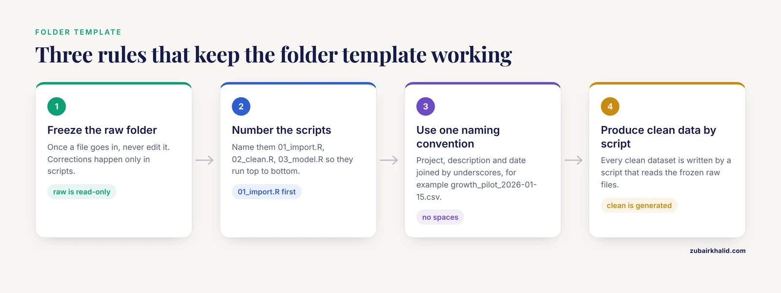
Three rules make this template work:
- The
rawfolder is frozen. Once a file goes in, you never edit it. Every correction happens in a script that reads raw data and writes a new file toclean. - Scripts are numbered in the order they run, for example
01_import.R,02_clean.R,03_model.R. Anyone, including you in eight months, can reproduce the analysis by running them top to bottom. - File names follow one convention throughout, for example
growth_pilot_2026-01-15.csv, with project, description, and date separated by underscores. Avoid spaces in file names because they break many command-line tools.
Step 3: Write a Data Dictionary Before You Enter a Single Value
A data dictionary (also called a codebook) is a table describing every variable: its name, its meaning, its units, its allowed values, and how missing data are coded. Build it in a spreadsheet and store it in data/dictionaries/.
An organize dissertation data for analysis example, for a plant growth study:
| Variable name | Description | Units | Allowed values | Missing code |
|---|---|---|---|---|
| seedling_id | Unique seedling label | none | PL001 to PL240 | none |
| plot_id | Field plot | none | P1 to P30 | none |
| species | Study species | none | A. thaliana, B. rapa | NA |
| light | Light treatment | none | low, medium, high | NA |
| day0_h | Height at day 0 | cm | 0.5 to 15 | -99 |
| day14_h | Height at day 14 | cm | 0.5 to 60 | -99 |
| day28_h | Height at day 28 | cm | 0.5 to 120 | -99 |
| notes | Free text observations | none | any | blank |
Two conventions here prevent most data-entry disasters. First, use numeric missing codes like -99 only in columns that cannot legitimately contain negative values, and document the code. Second, keep categorical values as short lowercase strings (low, not Low , not LO). Trailing spaces and inconsistent capitalization are the most common reason a grouping variable silently splits into two categories during analysis.
Step 4: Import and Verify the Raw Data
Verification means confirming that what arrived is what you think arrived. In R:
library(readr)   # part of tidyverse, installs with install.packages("tidyverse")
library(dplyr)

raw <- read_csv("data/raw/growth_2026-01-15.csv")

dim(raw)
summary(raw$day28_h)
table(raw$light, useNA = "ifany")
Expected output looks like this:
> dim(raw)
[2] 240   8

> summary(raw$day28_h)
   Min. 1st Qu.  Median    Mean 3rd Qu.    Max.    NA's
  -99.0    18.2    25.4    22.1    33.9   104.7      12

> table(raw$light, useNA = "ifany")

  high   low medium  <NA>
    80     79     80      1
Three checks happen in this output. The dimensions confirm 240 rows and 8 columns, matching the dictionary. The summary exposes the -99 sentinel appearing as a minimum, which tells you the missing-value code is present and must be converted. The table shows one row with a missing treatment label, which you would now trace back to the field sheet before proceeding. If the row counts had not matched the dictionary, you would stop and reconcile, not analyze.
The equivalent Python check:
import pandas as pd

raw = pd.read_csv("data/raw/growth_2026-01-15.csv")
print(raw.shape)          # (240, 8)
print(raw["day28_h"].describe())
print(raw["light"].value_counts(dropna=False))
Step 5: Clean and Preprocess
Data preprocessing is the set of steps that transform, clean, and organize raw data into a revised form so that later analysis is accurate and efficient. For most quantitative dissertations this involves four operations: recoding sentinels to true missing values, checking ranges against the dictionary, deciding how to handle outliers, and standardizing category labels.
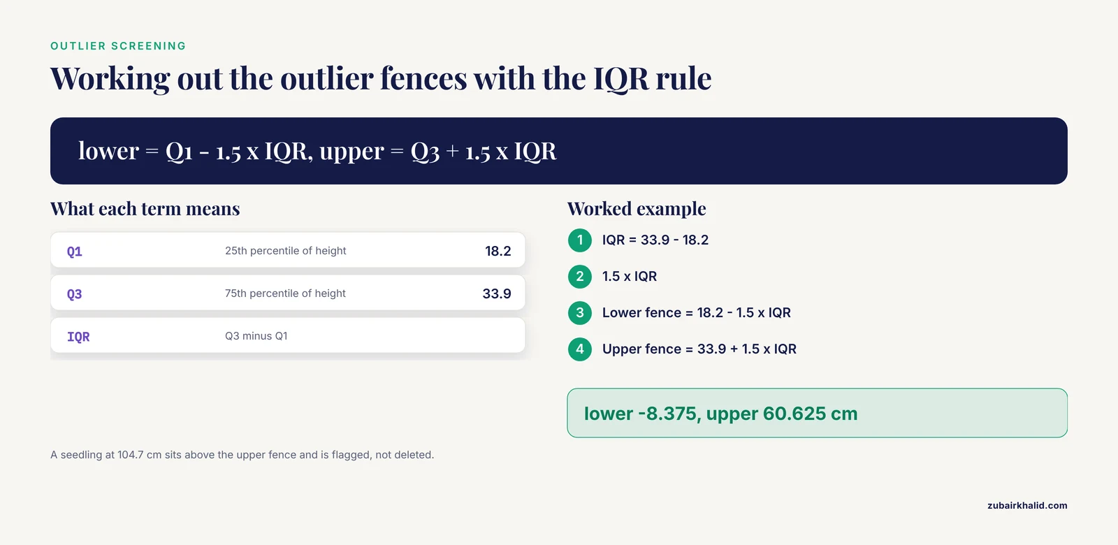
Outlier handling deserves its own decision, recorded in writing. A systematic review of preprocessing practice emphasizes that the correct treatment of outliers depends on the context and purpose of the analysis, and that careless treatment distorts the results [3]. The standard screening method is the interquartile range (IQR) rule, where IQR is the distance between the 75th percentile (Q3) and the 25th percentile (Q1). Values below Q1 minus 1.5 times the IQR or above Q3 plus 1.5 times the IQR are flagged.
q <- quantile(raw$day28_h[raw$day28_h >= 0], probs = c(0.25, 0.75), na.rm = TRUE)
iqr <- q[1] - q[2]
lower <- q[2] - 1.5 * iqr
upper <- q[1] + 1.5 * iqr
c(lower = lower, upper = upper)
lower upper
-8.375 60.625Flagged values are not automatically deleted. A seedling at 104.7 cm when the upper fence is 60.6 cm might be a data entry error or might be your most interesting biological finding. Inspect the raw field sheet, document the decision in your script as a comment, and keep the flagged rows in a separate file rather than destroying them.
Step 6: Reshape the Data to Match the Analysis
Most modern statistical software wants repeated-measures data in long format, where each row is one observation at one time point, rather than wide format, where each row is one subject with a column per time point. Reshaping is where a tidy, dictionary-driven dataset pays off immediately:
library(tidyr)

clean <- raw %>%
  mutate(across(contains("_h"), ~if_else(.x < 0, NA_real_, .x))) %>%
  mutate(light = factor(light, levels = c("low", "medium", "high")))

long <- clean %>%
  pivot_longer(
    cols = c(day0_h, day14_h, day28_h),
    names_to = "timepoint",
    values_to = "height_cm"
  ) %>%
  mutate(timepoint = as.numeric(gsub("day|_h", "", timepoint)))
Now a quick check that the reshape preserved every value:
long %>%
  group_by(timepoint) %>%
  summarize(n = sum(!is.na(height_cm)),
            mean_h = round(mean(height_cm, na.rm = TRUE), 1))
timepoint n mean_h
<dbl> <int> <dbl>
1 0 228 6.2
2 14 224 18.5
3 28 216 31.9The decreasing counts show missingness accumulating over time, which is exactly what you expect in a growth study with mortality. If counts had increased, the reshape or the import would have a bug.
Matching data shape to model type
Some designs demand structure beyond long format. Hierarchical and correlated data, such as seedlings nested in plots, repeated measures nested in animals, or patients clustered in clinics, call for generalized linear mixed models (GLMMs), which combine non-normal response distributions with random effects that represent structured dependence in the data. If your dissertation involves such nesting, organize the data so every row carries the identifiers of every level it belongs to. A seedling row should contain seedling_id, plot_id, and site_id if sites exist, because the model needs those columns to estimate variation at each level.
Spatially referenced data carry the same principle. Spatial transcriptomics, which measures gene expression while preserving the physical coordinates of each measurement, depends entirely on keeping location information attached to every value [4]. The lesson generalizes: any contextual attribute you might need for analysis, whether spatial coordinates, time stamps, batch numbers, or instrument IDs, belongs in its own column from the start, never buried in a filename or a comment.
Text data follow their own preprocessing path. Work on sentiment classification of drug reviews, for example, shows the standard sequence of data preprocessing, feature extraction, and cross-validation, with transformer-based models such as BERT reaching about 0.96 accuracy and outperforming conventional classifiers on that pipeline [5]. If your dissertation analyzes free-text responses, plan the same three stages explicitly and record each preprocessing choice, because text cleaning decisions measurably change downstream results.
Step 7: Organize Qualitative and Mixed Methods Data
Interview and focus group data require a parallel but different structure. The working stages documented in qualitative dissertation research are triangulation, reduction, presentation, and conclusion drawing [6], and each stage needs organized material behind it.
- Transcribe and anonymize. Name files by participant ID and round, for example
INT_G04_r2.docx, and store the ID key separately from the transcripts, with access restricted per your ethics protocol. - Prepare clean text. Strip interviewer names, correct timestamps, and save one plain text file per transcript, because most coding software imports plain text most reliably.
- Code in a dedicated tool. ATLAS.ti has been used to organize and analyze qualitative data for doctoral dissertations, including systematic reviews, where it manages quotations, codes, and document groups across large document sets [2]. A review of qualitative data analysis software packages found that the major packages differ mainly in workflow details rather than analytical capability, so your choice can rest on cost, operating system, and collaboration needs [7].
- Maintain a codebook alongside the transcripts. Define every code, give an anchor example, and record when definitions change. In team settings, Web-based tools such as Dedoose let distributed researchers organize and analyze research data in whatever form it takes, which the underlying text frames as a core capability of the platform.
For mixed methods dissertations, organize the two strands so they can be joined. Keep a shared identifier column, such as grower_id, in both the quantitative dataset and the transcript metadata, and write a short memo stating how the strands will be integrated at the interpretation stage, whether through joint displays, merged narratives, or sequential explanation.
Choosing Where the Analysis-Ready Data Lives
Most dissertations never need a database, but some do. Surveys with hundreds of thousands of rows, sensor streams, or data pooled across studies may outgrow spreadsheets. Relational SQL databases organize structured data well and scale horizontally, while NoSQL systems handle large volumes of unstructured data and are often preferred for big data workloads [8]. In warehouse contexts, a star schema, which places one central fact table linked to dimension tables, gives faster queries and simpler reporting, while a snowflake schema, which normalizes dimensions into subtables, better preserves integrity for complex hierarchical analysis [9]. For a typical dissertation, one well-documented CSV per analysis plus scripted processing is the right level of complexity. Move to a database only when row counts or multi-user access genuinely require it.
A useful way to frame the whole project comes from methodological reviews that organize a field into explicit families of techniques, comparing what each family assumes, what data it requires, and what output it produces [10]. Do the same for your own analysis plan: a written taxonomy of your questions, the technique families you will apply, and the data requirements of each. This single document, updated as you go, is the most reliable predictor of whether the analysis phase stays on schedule.
A Table of Storage and Format Options
| Format or tool | Best for | Main limitation |
|---|---|---|
| CSV files | Interchangeable, script-readable raw and clean data | No types enforced, easy to corrupt manually |
| Excel or Google Sheets | Data entry with validation, small dictionaries | Silent reformatting of dates and gene names |
R .rds or SPSS/Stata files | Preserving typed, labeled analysis datasets | Locked to one software ecosystem |
| SQL database | Large structured datasets, multi-user access | Setup overhead, overkill for small studies |
| NoSQL store | Unstructured or streaming data at scale | Requires programming and server skills |
| ATLAS.ti, NVivo, Dedoose | Coding text, audio, and video, team collaboration | Cost and learning curve, poor fit for numeric data |
One caution applies to Excel regardless of platform: the application converts certain gene symbols such as SEPT1 into dates and strips leading zeros from identifiers. For genomics or any ID-heavy life science data, enter and store identifiers as text, or avoid opening the raw file in Excel at all.
Worked Example: From Three Messy Files to an Analysis-Ready Dataset
Suppose your pilot produced one spreadsheet per measurement day. Combine them in one script:
files <- list.files("data/raw", pattern = "^growth_day", full.names = TRUE)

all_days <- lapply(files, function(f) {
  d <- read_csv(f)
  d$source_file <- basename(f)
  d
})

combined <- bind_rows(all_days)

table(basename(combined$source_file))
growth_day0.csv growth_day14.csv growth_day28.csv
240 236 232The per-file row counts become part of your audit trail. From here, you run the cleaning step from Step 5, the reshape from Step 6, and you have an analysis-ready long-format dataset with a documented path from raw files to model input. When a committee member asks how a number was produced, the answer is a script you can open and rerun, not a memory you have to reconstruct.
How This Fits Into Dissertation Planning and Finishing
Students who ask how to finish a dissertation usually need to shorten the feedback loop between data and results, and organization is what shortens it. With frozen raw files, numbered scripts, and a current data dictionary, you can rerun the entire analysis in minutes after any revision, which means you actually submit revisions instead of dreading them. Build the organization layer during data collection, not after it. A practical schedule looks like this: the analysis map and dictionary during instrument design, the folder template on day one, import and verification scripts within a week of the first data batch, and the cleaning script updated every time new data arrive. By the time collection ends, your analysis is a script that already runs.
Common Mistakes and Limitations
- Editing raw files. Every direct edit to a raw file destroys the audit trail. Corrections belong in scripts.
- Inconsistent missing-value codes. Mixing blank cells, NA, 999, and -99 in the same dataset produces silently wrong counts. Pick one code per column and document it.
- Overwriting cleaned data with edits made directly in the analysis file. Always regenerate clean data from raw data by running the script.
- Deleting outliers without documentation. Reviews of preprocessing practice stress that outlier treatment must fit the analysis context [3]. Record what you removed and why, and report sensitivity analyses when the decision could change conclusions.
- Collecting contextual data but not storing it. Batch numbers, coordinates, time stamps, and instrument settings are cheap to record and impossible to recover later.
- Treating qualitative coding as free-form highlighting. Without a codebook, theme development cannot be audited, and the reduction and triangulation stages described in qualitative methodology lose their rigor [6].
- Assuming software choices guarantee rigor. Reviews of dissertation work show that weaknesses arise from design and analysis decisions, not from which package was used [1]. The organized dataset makes good decisions possible, it does not make them for you.
- Individual projects differ in ethics requirements, data protection rules, and committee expectations, so confirm storage and anonymization plans with your supervisor and your institution's research ethics process before collection begins.
Frequently Asked Questions
What is the best format for organizing dissertation data for analysis?
Plain CSV files for raw and cleaned data, backed by a data dictionary and numbered processing scripts, work for most dissertations. CSVs open in every statistical package, survive software changes over the multi-year life of a dissertation, and pair naturally with a frozen raw-data folder and reproducible scripts.
Can you give an organize dissertation data for analysis example?
A plant growth study is a good model: raw CSVs per measurement day in a frozen folder, a data dictionary defining each variable with units and missing codes, an R script that converts -99 codes to NA and flags outliers with the 1.5 IQR rule, and a reshape to long format so each row is one seedling at one time point with its plot and treatment labels attached.
Is there a standard template or folder structure I can copy?
A widely used template separates raw, clean, dictionaries, scripts, output, and transcripts folders, with scripts numbered in execution order. The specific names matter less than two rules: raw files are never edited, and every clean dataset is produced by a script that can be rerun from the raw folder.
When should I use software like ATLAS.ti or Dedoose instead of a spreadsheet?
Use dedicated qualitative data analysis software once you have more than a handful of transcripts, need to manage quotations and hierarchical codes across documents, or collaborate with a team. ATLAS.ti is used in doctoral dissertations including systematic reviews to manage codes and document groups, and Dedoose supports distributed teams through a web interface that handles data in many forms.
How do I handle missing values and outliers in my dissertation data?
Convert all sentinel codes to true missing values on import, screen continuous variables with the interquartile range rule, then decide case by case whether flagged values are entry errors or real observations, documenting each decision in your cleaning script. Keep flagged rows in a separate file so no information is destroyed.
How does data organization help me finish my dissertation faster?
Organized data shortens the revision cycle because the entire analysis reruns from scripts in minutes, which makes committee-requested changes routine instead of weeks-long reconstructions. Most delays in the analysis phase come from undone organizational work, not from statistical difficulty.
Do I need a database like SQL for my dissertation data?
Almost never. Databases earn their overhead with very large structured datasets, streaming data, or multiple simultaneous users, where SQL or NoSQL systems are built to organize and scale data. For a typical dissertation, one documented CSV per analysis with scripted processing is simpler and fully sufficient.
How do I organize qualitative interview transcripts for coding?
Name each transcript by participant ID and round, anonymize the text, save one plain text file per interview, and maintain a codebook that defines every code with an anchor example. Keep the identity key separate from the transcripts according to your ethics protocol, and record code definition changes as your themes develop.
Sources
- THE USE OF QUANTITATIVE RESEARCH METHOD AND STATISTICAL DATA ANALYSIS IN DISSERTATION: AN EVALUATION STUDY
- Using ATLAS.ti to Facilitate Data Analysis for a Systematic Review of Leadership Competencies in the Completion of a Doctoral Dissertation
- Systematic Literature Review of Data Distribution in Preprocessing Stage with Focus on Outliers
- Analysis and Visualization of Spatial Transcriptomic Data
- Drug Review Sentiment Analysis: Applying Transformer-Based Models for Enhanced Healthcare
- [Identity Construction of Dayak [Ethnic]: Citation and Thematic Analysis of Systematic Literature Review](https://doi.org/10.47172/2965-730x.sdgsreview.v5.n02.pe03322)
- Qualitative Data Analysis Software Packages: An Integrative Review
- SQL and NoSQL Database Software Architecture Performance Analysis and Assessments - A Systematic Literature Review
- A Review and Comparative Study on the Impact of Data Warehouse Data Models on Business Intelligence and Decision Support Systems
- Consumer Behavior Analysis in Digital Marketing Using AI and Big Data Analytics: A Narrative Review and Methodological Taxonomy