Open Source Data Visualization Tools for Reproducible Research
By Dr. Zubair Khalid, DVM, MS, PhD ·

By the end of this article you will be able to build a publication-quality figure from raw data using free, open source data visualization tools, save that figure with code instead of manual edits, and prove to a collaborator (or a reviewer, or yourself in eight months) that the exact same figure can be regenerated from the exact same files with one command. You will also get a reproducibility checklist you can apply to any figure, dataset, or analysis pipeline.
Before you start, have the following on hand:
- Python 3.10 or newer, installed through Miniconda or Anaconda (Windows, macOS, or Linux)
- Git for version control
- A plain text editor or IDE such as VS Code
- A small CSV dataset, either your own or any export from a plate reader, qPCR run, flow cytometer, or public repository
What Reproducibility Means for a Figure
Reproducible research means that another person, working from your raw data and your code, can produce your results without contacting you. For a figure, this has a precise definition: every visible element (the points, the axis limits, the colors, the statistical annotations) is determined by code that runs on the raw data, not by anything you dragged with a mouse.
The microscopy community makes the case clearly. The Nion Swift project, an open source Python package for controlling electron microscopes and visualizing spectrum imaging data, states the principle directly: visualization, processing, and analysis tools must be able to be shared, reported upon, and reused months or years later, and to trust that workflow the tools must be readily available and transparent in their functionality [1]. Closed, click-driven software fails that test because the "how" lives in a human's memory rather than in a script.
The same principle applies to data cleaning. The ODM Tools Python application, built for hydrologic and water quality sensor data, automatically records every manual quality control edit as a Python script, preserving the provenance of the corrections so the entire data editing chain stays traceable and reproducible [2]. That design solves a problem biologists face constantly: figures built on hand-corrected data cannot be reproduced because nobody recorded which points were removed or why.
Open source data visualization for reproducible research works because two properties come together. The source code is inspectable, so nothing about the rendering is a black box. And the tool is free, so a reviewer or collaborator can run your exact pipeline without a license.
The Open Source Toolchain at a Glance
Most reproducible visualization work in the life sciences falls into two layers: general-purpose plotting libraries you script directly, and domain-specific packages built on top of them for particular data types.
| Tool | Language | What it visualizes | Notes |
|---|---|---|---|
| Matplotlib | Python | General 2D plots, publication figures | Foundation of most Python plotting, scriptable and deterministic |
| Seaborn | Python | Statistical graphics built on Matplotlib | Dataframe-aware, concise syntax |
| Plotly / D3 | Python / JavaScript | Interactive web figures | D3 drives visualization in real-time big data pipelines |
| ggplot2, Shiny | R | Statistical graphics, interactive web apps | Shiny hosts apps such as NeuroVar [3] |
| pyActigraphy | Python | Actigraphy (rest-activity) data | Reads multiple formats, sleep agendas, rhythm variables [4] |
| Visbrain | Python | Multimodal brain data, GPU-accelerated | Object layer plus GUIs for EEG, MEG, MRI [5] |
| Sleep | Python | Polysomnography, hypnograms, spectrograms | Automatic spindle and K-complex detection, publication-ready tables [6] |
| BRAVO | Python (web) | Deep brain stimulation recordings | Browser interface for longitudinal neural data [7] |
| Osprey-MRSI | MATLAB/Python ecosystem | Magnetic resonance spectroscopic imaging | Automated pipeline with interactive HTML quality-control reports, NIfTI-MRS export [8] |
| GITAR (HiCtool) | Python | Hi-C chromatin contact matrices and TADs | Step-by-step pipeline from raw data to contact matrices [9] |
| Vayu | R | Air quality and other time-series sensor data | Combines visualization with statistical analysis in one GUI [10] |
| GenomeGraphR | R (web app) | Foodborne pathogen whole genome sequencing data | Tested on 160,000 sequenced isolates from NCBI Pathogen Detection [11] |
| QGIS | C++/Python (GUI) | Geographic and relief data | Free and open source GIS for terrain visualization [12] |
| FREEWAT | QGIS plugin | Groundwater and surface-water models | Couples GIS post-processing with MODFLOW-family simulation codes [13] |
The domain-specific entries matter because they demonstrate a pattern: when researchers need reproducible visualization of a specialized data type, they increasingly publish a scriptable package rather than a point-and-click program. pyActigraphy, for example, was built to handle the growing analysis of large population-based actigraphy samples, reading many vendor formats and quantifying rest-activity rhythm variables in scripted workflows [4]. Visbrain follows the same philosophy, separating configurable visual objects (a 3D brain, connectivity sources) from graphical interfaces, in a design explicitly modeled on Matplotlib's subplot approach so figures can be produced automatically [5].
Public data resources reinforce this shift. Large publicly funded projects now generate multi-assay genomic datasets spanning sequencing, RNA and microRNA profiling, and proteomics, and the analysis ecosystem around them is built on explicitly open, integrative visualization tools [14]. Learning the general-purpose layer first means every one of these domain packages becomes easier to read, extend, and trust.
Step-by-Step: Build a Reproducible Figure Pipeline
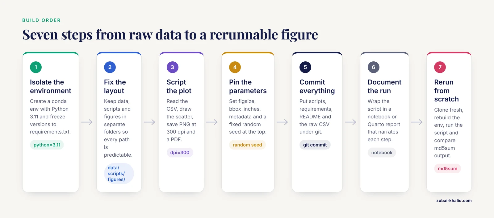
This walkthrough builds a complete, regenerable figure pipeline. Follow the steps in order in your terminal.
Step 1: Create an isolated environment
Isolation guarantees that your figure depends on known package versions, not on whatever happens to be installed system-wide.
conda create -n figenv python=3.11
conda activate figenv
pip install pandas matplotlib seaborn
Now freeze the exact versions:
pip freeze > requirements.txtEach line of requirements.txt follows the pattern package==version, for example pandas==2.2.3 (replace with the version pip reports on your machine). Anyone can rebuild your environment with:
pip install -r requirements.txtStep 2: Lay out the project
Use a fixed directory structure so every script path is predictable:
my-project/
    data/
        measurements.csv
    scripts/
        plot_fig1.py
    figures/
    requirements.txt
    README.md
The raw data lives in data/, every figure is written to figures/, and nothing is ever overwritten by hand.
Step 3: Write the plotting script
Create scripts/plot_fig1.py:
import pandas as pd
import matplotlib.pyplot as plt

df = pd.read_csv("data/measurements.csv")
print(df.info())

fig, ax = plt.subplots(figsize=(4, 3), constrained_layout=True)
ax.scatter(df["concentration_um"], df["response"],
           s=20, color="#2171b5", alpha=0.8)
ax.set_xlabel("Concentration (uM)")
ax.set_ylabel("Response (a.u.)")
ax.spines["top"].set_visible(False)
ax.spines["right"].set_visible(False)

fig.savefig("figures/fig1_scatter.png", dpi=300)
fig.savefig("figures/fig1_scatter.pdf")
Run it from the project root:
python scripts/plot_fig1.pyExpected output in the terminal:
<class 'pandas.core.frame.DataFrame'>
RangeIndex: 24 entries, 0 to 23
Data columns (total 2 columns):
 #   Column           Non-Null Count  Dtype
---  ------           --------------  -----
 0   concentration_um  24 non-null     float64
 1   response          24 non-null     float64
And two new files appear: figures/fig1_scatter.png (300 dpi raster for slides) and figures/fig1_scatter.pdf (vector for journals). Every pixel and every curve traces back to the CSV and the script.
Step 4: Understand the parameters that control reproducibility
| Parameter | Where | What it controls | Recommended setting |
|---|---|---|---|
dpi | savefig | Raster resolution in dots per inch | 300 for print, 150 for drafts |
figsize | plt.subplots | Physical figure size in inches | Match the target column width (often 3.5 in single, 7 in double) |
bbox_inches | savefig | Whether the saved figure is cropped | "tight" trims whitespace, but changes output dimensions between versions, so pin it deliberately |
format | savefig | Output file type from the extension | Save both PDF (vector) and PNG (raster) |
metadata | savefig | Embedded author, title, date strings | Set explicitly so embedded metadata does not vary between runs |
| random seed | numpy.random.seed | Randomness in sampling, jitter, bootstraps | Set a fixed integer at the top of the script |
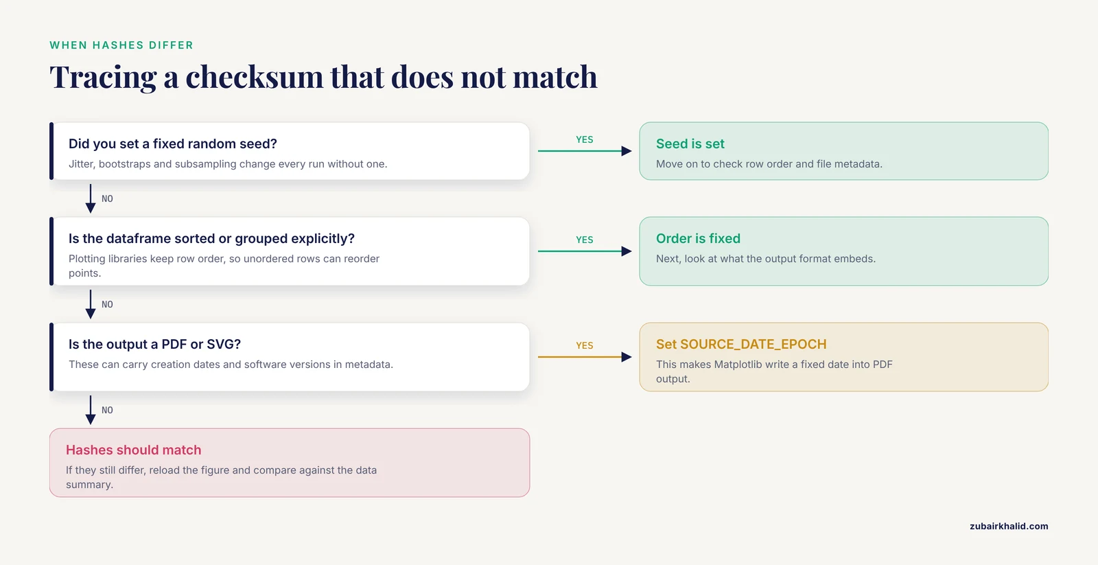
Two other settings prevent silent nondeterminism. Set plt.rcParams["axes.unicode_minus"] = False if your target font lacks the Unicode minus sign, and always sort or group your dataframe explicitly before plotting, because plotting libraries preserve row order and unordered rows can reorder points between runs on different machines.
Step 5: Version control the whole pipeline
git init
git add scripts/ requirements.txt README.md data/measurements.csv
git commit -m "Add reproducible figure 1 pipeline"
Now every change to the figure has a timestamped, revertable record. If a reviewer asks for the previous axis scaling, git log and git checkout recover it in seconds.
Step 6: Document with a notebook or generated report
Wrap the script in a Jupyter notebook or Quarto document that narrates each step. Domain packages show how far this can go: Osprey-MRSI pairs its fully automated spectroscopic imaging pipeline with interactive HTML reports so a reader can inspect every processing step, alongside exports in NIfTI-MRS format for use in other toolboxes [8]. Your notebook serves the same purpose at smaller scale: narrative, code, and rendered figure in one artifact that runs top to bottom.
Step 7: Run the rerun-from-scratch test
This is the proof. On a clean machine (or a fresh directory), repeat the entire chain:
git clone <your-repository-url>
cd my-project
conda create -n figenv python=3.11
conda activate figenv
pip install -r requirements.txt
python scripts/plot_fig1.py
md5sum figures/fig1_scatter.png
Compare the checksum printed by md5sum against the one from your original machine (md5sum figures/fig1_scatter.png there too). Identical hashes mean byte-for-byte reproduction. If they differ, check for randomness you forgot to seed, unsorted data, or PDF creation-date metadata (setting the SOURCE_DATE_EPOCH environment variable makes Matplotlib write a fixed date into PDF output).
Common Errors, Exact Messages, and Fixes
ModuleNotFoundError: No module named 'pandas'. Your terminal is not using the project environment. Runconda activate figenvand confirm withwhich python(macOS/Linux) orwhere python(Windows) that the interpreter lives inside the environment.FileNotFoundError: [Errno 2] No such file or directory: 'data/measurements.csv'. You launched the script from the wrong directory. Paths are resolved relative to where you run Python, not where the script file sits.cdto the project root, or build paths frompathlib.Path(file).parent.KeyError: 'concentration_um'. The column name in the script does not match the CSV. Print the real names withprint(df.columns.tolist())and fix the spelling, including stray spaces, whichdf.columns = df.columns.str.strip()removes.Glyph 8722 (\N{MINUS SIGN}) missing from current fontin the render output. A Unicode minus sign appears in a tick label and your font cannot render it. Setplt.rcParams["axes.unicode_minus"] = False.- Plots accumulating across script runs and slowing to a crawl. Each
plt.subplots()call opens a new in-memory figure. Callplt.close(fig)after saving, especially in loops.
To check that a saved figure is actually right, never judge from memory. Reload it (open the PNG, or the PDF in any viewer) and compare against a printed summary of the data: the number of plotted points should equal len(df) after any documented filtering, and axis limits should bracket the min and max of the plotted columns, which you can verify with df["response"].min() and df["response"].max().
Domain Tools Worth Knowing Before You Need Them
Specialized open source packages save enormous time once your data matches their formats, and knowing they exist changes how you plan an analysis.
For neurophysiology, Visbrain provides GPU-accelerated 2D and 3D rendering for intracranial EEG, scalp EEG, MEG, and MRI data, built in tight collaboration with neuroscientists so the tools stay transparent to the recording modality [5]. Its Sleep module adds a full GUI for polysomnographic visualization, scoring, automatic spindle and K-complex detection, and publication-ready descriptive tables, loading standard formats such as European Data Format (EDF) [6]. For deep brain stimulation recordings, BRAVO offers a browser-based interface that parses session files from clinical programming tablets and organizes neural recordings for longitudinal analysis [7].
For genomics, GITAR leads users step by step from raw Hi-C data through normalization to intra-chromosomal contact matrices and topologically associated domain coordinates, with a library of standardized processed human and mouse datasets so different experiments can be compared consistently [9]. GenomeGraphR integrates whole genome sequencing data with curated epidemiological metadata in a web interface built for querying transmission sources and dynamics across time and space [11]. NeuroVar, implemented as both an interactive Shiny application and a standalone desktop app, visualizes genetic variation and gene expression profiles for neurological disease biomarkers, distributed through its GitHub repository [3]. For environmental and spatial data, Vayu bundles visualization, interpolation, aggregation, and prediction for sensor time series in one cross-platform toolbox [10], while QGIS supports relief visualization techniques that combine hillshading with layers derived from digital elevation models [12], and the FREEWAT plugin couples QGIS spatial analysis with distributed groundwater simulation codes [13].
Even fields far from biology use the same pattern. ReciPro brings free, open source crystallographic visualization with a built-in database of over 20,000 crystal models and real-time diffraction simulation [15], and VINE gives neuroevolution researchers interactive views of agent behavior across training generations. TB Mobile applies open source molecular fingerprints to visualize compound-target relationships for tuberculosis drug discovery on mobile platforms [16]. When you inherit a new data type, searching for "(data type) open source visualization" almost always turns up a maintained package, and open standards underlie several of these systems, including standard-based medical data visualization [17].
Tips for Open Source Data Visualization
- Separate data, code, and output directories from day one. If a figure can only be regenerated when files sit in their original arrangement, the pipeline is not reproducible.
- Pin versions, not just package names.
pandasin requirements.txt without a version number invites silent behavior changes across releases. - Save figures in vector format for publication. PDF and SVG scale without pixelation and keep text selectable, with PNG alongside for slides.
- Script the cleaning, not just the plotting. Follow the ODM Tools precedent and record every data correction as code so the editing chain itself is auditable.
- Write one function per figure. A function like
def plot_fig1(df, outdir)returns a figure from a dataframe, which makes it testable and reusable across projects. - Use a style sheet.
plt.style.use("seaborn-v0_8-whitegrid")or your own.mplstylefile keeps fonts, tick sizes, and line widths consistent across every figure in a manuscript. - Read the domain package's documentation before writing your own parser. pyActigraphy alone implements methods for reading multiple actigraphy formats, automatic rest-period detection, and multiple sleep detection algorithms, work you should not repeat [4].
Common Mistakes and Limitations
- Hand-editing final figures in drawing software. Moving a label in Inkscape or Illustrator breaks the link between code and output. If a figure needs an annotation, add it in the plotting script.
- Saving over the only copy of raw data. Scripts should read raw files and write derived files, never modify
data/in place. - Relying on interactive GUI state. A figure produced after twenty undocumented clicks in a GUI tool cannot be reproduced. GUI tools such as Visbrain and Sleep are excellent for exploration, but export the final figure through a scripted call or save the session parameters [5], [6].
- Unseeded randomness. Bootstrapped confidence intervals, jittered scatter points, and random subsampling change every run unless you set a seed. Reviewers regenerating your figure will see different error bars and lose trust.
- Assuming the fresh-machine test once. Run the rerun-from-scratch test after every major change, not just before submission. Dependencies drift, and a pipeline that passed in March can fail in September.
- Mixing environments across projects. Installing everything into one shared environment guarantees that upgrading a package for one project breaks another. One environment per project is the norm.
- Overlooking file format nondeterminism. Some output formats embed timestamps or software versions in their metadata. PNG output from Matplotlib is generally stable, while PDF and SVG can carry creation dates, which is why the checksum test and
SOURCE_DATE_EPOCHmatter. - A practical limitation of open source tools. Domain packages vary in documentation depth and maintenance activity, and a package with a small user base may stop receiving updates. Check the repository's recent commit history before building a thesis on top of one. Individual data quirks, unusual instruments, or project-specific regulatory requirements may also need expert consultation beyond any published tool.
Your Reproducibility Checklist
Run every figure and analysis through this list before you share it:
- Raw data files are read-only and stored in a
data/directory that scripts never modify. - All cleaning, filtering, and quality control edits exist as code, not as undocumented manual changes.
- Every figure is produced by a script, with no manual post-editing.
- All random operations have fixed seeds.
- Package versions are pinned in
requirements.txtor an equivalent environment file. - The environment can be rebuilt from that file alone on a clean machine.
- Running the full pipeline from a fresh clone regenerates every figure without errors.
- Checksums of regenerated output match the originals (where format metadata allows exact comparison).
- The project includes a README stating which script produces which figure, and the expected run order.
- Data provenance is recorded, including where public data came from and on what date it was downloaded.
Frequently Asked Questions
What counts as an open source data visualization tool?
Any tool whose source code is publicly available under a license that permits use, modification, and redistribution, and which produces graphics from data. Matplotlib, Seaborn, ggplot2, QGIS, and domain packages such as pyActigraphy all qualify. Point-and-click software with closed source code does not, regardless of whether it is free to use.
Do I need to learn Python or R to use these tools?
For the general-purpose libraries, yes at a basic level, because reproducibility comes from scripting. However, many domain packages lower the barrier considerably: GITAR is designed so users without programming or bioinformatics expertise can work with Hi-C data [9], and NeuroVar, BRAVO, and Vayu all provide graphical interfaces on top of their engines.
What is the difference between reproducible and replicable research?
Reproducibility means the same team's data and code give the same result when re-run. Replicability means a different team, with new data, reaches consistent conclusions. Visualization pipelines strengthen both, but the rerun-from-scratch test described in this article addresses reproducibility specifically.
How do I choose between Matplotlib, ggplot2, and Plotly?
Match the language your analysis already uses, since moving data between languages introduces errors. Matplotlib dominates Python scientific publishing, ggplot2 dominates R, and Plotly suits interactive or web-embedded figures. All three are open source and scriptable, so all three satisfy reproducibility requirements.
How do I make a figure reproducible if I already edited it by hand?
Rebuild it as code. Identify each manual change (color, annotation, crop), translate each into a plotting parameter, and rerun. It usually takes under an hour for a standard panel and permanently removes the figure from the category of things that only exist once.
What belongs in a reproducibility checklist?
Raw data preservation, scripted cleaning and plotting, pinned dependencies, fixed random seeds, a version-controlled repository, a successful rerun on a clean machine, and a README explaining the run order. The ten-item checklist in this article covers the standard set.
Can open source visualization tools handle clinical or regulated data?
Yes, provided you control where the data goes. Open source tools running locally on your own hardware never upload anything, which is an advantage over many web services. Published examples include open source visualization applied to standard-based medical data [17] and the BRAVO platform, built specifically for clinical and research use with deep brain stimulation recordings [7]. Always follow your institution's data governance rules before moving patient data anywhere.
How do I share figures so others can regenerate them?
Share the entire repository: raw data, scripts, requirements file, and README, through GitHub or Zenodo. A collaborator who can clone it, create the environment from requirements.txt, and run the scripts has everything needed. For publication, archive the repository with a permanent identifier so the link in your paper does not decay.
Sources
- Nion Swift: Open Source Image Processing Software for Instrument Control, Data Acquisition, Organization, Visualization, and Analysis Using Python.
- Open source software for visualization and quality control of continuous hydrologic and water quality sensor data
- NeuroVar: an open-source tool for the visualization of gene expression and variation data for biomarkers of neurological diseases
- pyActigraphy: Open-source python package for actigraphy data visualization and analysis
- Visbrain: A Multi-Purpose GPU-Accelerated Open-Source Suite for Multimodal Brain Data Visualization
- Sleep: An Open-Source Python Software for Visualization, Analysis, and Staging of Sleep Data
- Brain Recording Analysis and Visualization Online (BRAVO): An open-source visualization tool for deep brain stimulation data.
- Fully automated open-source analysis and interactive visualization of magnetic resonance spectroscopic imaging (MRSI) data in Osprey-MRSI.
- GITAR: An Open Source Tool for Analysis and Visualization of Hi-C Data
- Vayu: An Open-Source Toolbox for Visualization and Analysis of Crowd-Sourced Sensor Data
- GenomeGraphR: A user-friendly open-source web application for foodborne pathogen whole genome sequencing data integration, analysis, and visualization
- Relief visualization techniques using free and open source GIS tools
- Integrating free and open source tools and distributed modelling codes in GIS environment for data-based groundwater management
- Public data and open source tools for multi-assay genomic investigation of disease
- ReciPro: free and open-source multipurpose crystallographic software integrating a crystal model database and viewer, diffraction and microscopy simulators, and diffraction data analysis tools
- New target prediction and visualization tools incorporating open source molecular fingerprints for TB Mobile 2.0
- Applying open source data visualization tools to standard based medical data.