White Test for Heteroskedasticity: Definition and Example

By Dr. Zubair Khalid, DVM, MS, PhD · 2026-10-03

The test de White is a statistical test that checks whether the variance of the errors in a regression model is constant, a property called homoskedasticity [1]. It detects both linear and nonlinear forms of heteroskedasticity, so it catches patterns that simpler tests miss. You run it by regressing the squared residuals on the fitted values and their squares, then testing whether those coefficients are jointly zero.

Quick Answer

The test de White tests the null hypothesis of constant error variance (homoskedasticity) against the alternative that variance changes with the predictors [1].
It works by regressing squared residuals on the fitted values and their squares, then forming an LM statistic from that auxiliary regression [2].
The statistic follows a chi-square distribution with 2 degrees of freedom in the fitted-value form.
A small p-value (below your significance level, often 0.05) means you reject homoskedasticity and suspect heteroskedasticity.
A large p-value means you fail to reject homoskedasticity, so the constant-variance assumption looks reasonable.

What the White Test Means

In plain terms, the test de White asks one question: does the spread of your regression errors stay the same across all predicted values, or does it grow and shrink? If the spread changes, your standard errors and confidence intervals can be wrong [3].

The precise statistical definition is this. Consider the linear model

$$y_i = \beta_0 + \beta_1 x_{i1} + \dots + \beta_k x_{ik} + u_i$$

The null hypothesis is that the error variance is constant, $H_0: \text{Var}(u_i \mid x_i) = \sigma^2$. The alternative is that the variance depends on the regressors in some way, including squared and cross-product terms [1]. Halbert White proposed the test in 1980, along with a heteroskedasticity-consistent covariance estimator that lets you keep valid standard errors even when the variance is not constant [1].

How It Works

The test uses an auxiliary regression. You take the residuals from your original model, square them, and regress those squared residuals on the fitted values and the squared fitted values [2]:

$$\widehat{u_i^2} = \delta_0 + \delta_1 \widehat{y_i} + \delta_2 \widehat{y_i^2} + \text{error}$$

Here is what each symbol means.

$\widehat{u_i^2}$ is the squared residual for observation $i$, a proxy for the error variance at that point.
$\widehat{y_i}$ is the fitted value from the original regression.
$\widehat{y_i^2}$ is that fitted value squared, which captures nonlinear variance patterns.
$\delta_0, \delta_1, \delta_2$ are the coefficients estimated in the auxiliary regression.

The null hypothesis is $H_0: \delta_1 = \delta_2 = 0$, meaning the squared residuals do not depend on the fitted values [2]. The test statistic is

$$LM = n \cdot R^2_{aux}$$

where $n$ is the sample size and $R^2_{aux}$ is the R-squared from the auxiliary regression. Under the null, this statistic follows a chi-square distribution with degrees of freedom equal to the number of restrictions, which is 2 in this fitted-value form. You can run this in Python with the het_white function from statsmodels.stats.diagnostic [1], in R with the white function from the skedastic package [1], or in Stata with estat imtest, white [1].

Worked Example

The dataset has 30 house prices (in thousands) regressed on size (thousands of square feet) and age (years).

size	age	price	size	age	price
1.2	5	210	3.4	6	375
1.5	10	235	1.6	11	240
1.8	3	260	2.3	19	300
2.0	20	255	2.9	13	345
2.2	8	290	1.3	16	215
2.5	15	310	1.9	21	270
2.7	2	330	2.6	17	320
3.0	25	300	3.3	23	365
3.2	12	355	1.1	24	200
3.5	7	370	2.05	26	280
1.4	18	225	2.45	27	315
1.7	4	250	2.75	28	335
2.1	22	285	3.15	29	350
2.4	9	305	3.45	30	360
2.8	1	340
3.1	14	360

Step 1: Fit the original model. The OLS regression gives

$$\text{price} = 132.6019 + 71.7704 \cdot \text{size} - 0.3202 \cdot \text{age}$$

with $R^2 = 0.9602$.

Step 2: Compute squared residuals. For each of the 30 observations, square the residual $e_i^2$.

Step 3: Run the auxiliary regression. Regress the squared residuals on the fitted values and their squares:

$$e^2 = -1041.3973 + 6.9092 \cdot \text{fitted} - 0.0100 \cdot \text{fitted}^2$$

The auxiliary R-squared is $R^2_{aux} = 0.0408$.

Step 4: Form the LM statistic.

$$LM = n \cdot R^2_{aux} = 30 \cdot 0.0408 = 1.2243$$

Step 5: Get the p-value. With 2 degrees of freedom, $P(\chi^2_2 > 1.2243) = 0.5422$.

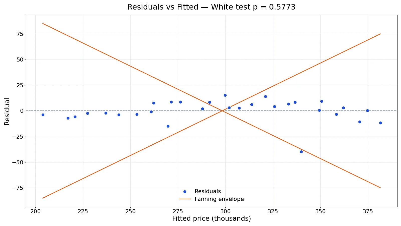
The statsmodels het_white function uses the full White specification with cross-product terms, so it reports a slightly different statistic: LM = 3.8085 with p = 0.5773. Both versions point the same way.

import statsmodels.api as sm
from statsmodels.stats.diagnostic import het_white
X = sm.add_constant(df[['size','age']])
model = sm.OLS(df['price'], X).fit()
lm, p, f, fp = het_white(model.resid, X)
print(f"LM = {lm:.4f}, p-value = {p:.4f}")

Output:

LM = 3.8085, p-value = 0.5773

How to Interpret It

The p-value is the probability of seeing a test statistic at least this extreme if the null hypothesis of constant variance were true [4]. A small p-value is evidence against homoskedasticity.

In the example, p = 0.5422 (or 0.5773 from statsmodels). Both are well above 0.05, so you fail to reject the null. There is no statistical evidence of heteroskedasticity in this regression, even though the residual plot shows some fanning. The test and the plot disagree here, which is a useful reminder that visual patterns can be noise in a small sample.

If the p-value had been below 0.05, you would reject homoskedasticity. You would then either model the variance explicitly or switch to heteroskedasticity-consistent standard errors, which keep your coefficient tests valid [1].

When to Use It (and when not to)

Use the test de White after fitting a linear regression when you want to check the constant-variance assumption before trusting standard errors, t-tests, or F-tests. It is a good default because it does not assume a specific form for the heteroskedasticity [1]. It pairs well with a residual plot, which shows you the shape of any problem.

Skip it when your sample is very small, because the chi-square approximation needs enough observations to be reliable. Skip it when you have already decided to report heteroskedasticity-consistent standard errors regardless, since the test then adds little. If you only suspect a linear variance pattern, the Breusch-Pagan test is a more targeted alternative [1]. For a broader guide to picking the right procedure, see statistical tests: choosing the right one for your data.

White Test vs Breusch-Pagan Test

Both tests check for nonconstant error variance, but they differ in what they can detect.

Feature	White test	Breusch-Pagan test
Detects linear heteroskedasticity	Yes	Yes
Detects nonlinear heteroskedasticity	Yes	No [1]
Auxiliary regressors	Fitted values, squares, cross products	Original regressors
Degrees of freedom	Depends on terms included	Number of regressors
Main weakness	Low power in small samples	Misses nonlinear patterns

The Breusch-Pagan test is designed to detect only linear forms of heteroskedasticity [1]. Under certain conditions and with a modification, the two tests can be algebraically equivalent [1]. If you want a single broad check, the White test covers more ground.

Common Mistakes

Reading a significant result as proof of heteroskedasticity only. A significant White statistic can also signal a specification error, such as a missing variable or wrong functional form [1]. Fix: check your model specification before blaming the variance.
Ignoring the version of the test you ran. The fitted-value form and the full cross-product form give different statistics. Fix: report which form you used and stay consistent.
Using the test on a tiny sample. The chi-square approximation is unreliable with few observations. Fix: treat results as suggestive and lean on residual plots.
Confusing the null hypothesis direction. The null is homoskedasticity, not heteroskedasticity. Fix: remember that a small p-value rejects constant variance.
Skipping the residual plot. The test gives a yes or no answer but no shape. Fix: always plot residuals against fitted values to see the pattern [3].
Applying it to non-linear models without care. The standard form assumes a linear regression. Fix: use a test designed for your model class.

Limitations

The test de White tells you whether variance is constant, but it cannot tell you the correct variance model or fix the problem for you. A significant result leaves you choosing between weighted least squares, a transformation, or heteroskedasticity-consistent standard errors [1]. It also cannot separate heteroskedasticity from specification error, so a rejection may point to a modeling mistake instead of a variance issue [1].

The test has low power in small samples and can miss real heteroskedasticity when the pattern is subtle. It can also reject the null for reasons unrelated to the error variance, such as outliers or non-normal errors. Treat it as one piece of evidence alongside plots and domain knowledge, not as a final verdict.

Frequently Asked Questions

What does the White test actually test?

It tests whether the variance of the regression errors is constant across observations [1]. The null hypothesis is homoskedasticity, and the alternative is that the variance depends on the regressors, including nonlinear terms. A small p-value means you reject constant variance.

What does a p-value above 0.05 mean for the White test?

It means you fail to reject the null hypothesis of constant variance. In the house-price example, p = 0.5422, so there is no statistical evidence of heteroskedasticity. This does not prove the variance is constant, it just means the data are consistent with that assumption.

Is the White test the same as the Breusch-Pagan test?

No. The Breusch-Pagan test detects only linear forms of heteroskedasticity, while the White test also catches nonlinear patterns [1]. Under certain conditions and a modification of one test, they can be algebraically equivalent [1]. The White test is the broader check.

How do I run the White test in Python?

Use the het_white function from statsmodels.stats.diagnostic [1]. Pass it the residuals and the design matrix from your fitted model. It returns the Lagrange multiplier statistic, the p-value, and the F-statistic version. The example above shows the exact call.

What should I do if the White test rejects homoskedasticity?

You have two main options. You can model the variance directly with weighted least squares, or you can keep your coefficients and report heteroskedasticity-consistent standard errors [1]. The second option is simpler and widely used. Either way, check whether a specification error is the real cause first [1].