What Is Heteroscedasticity? Definition and Examples
By Dr. Zubair Khalid, DVM, MS, PhD ·
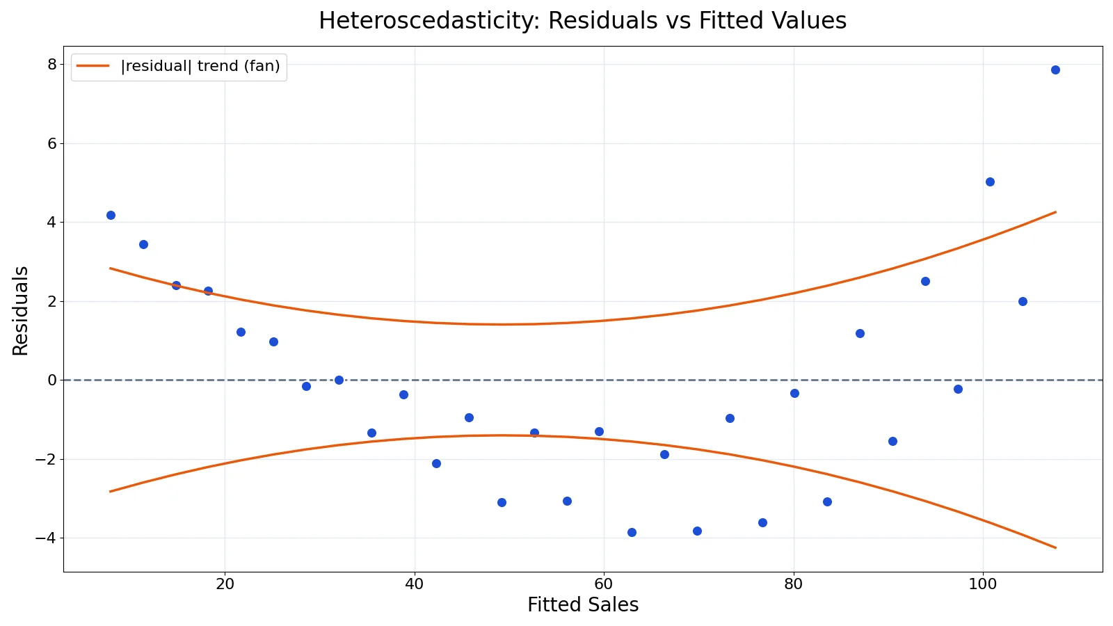
Heteroscedasticity is the condition in which the variance of the errors in a regression model is not constant across observations. In plain terms, your model predicts some values well and others poorly, and the size of those misses grows or shrinks in a pattern. It does not bias the ordinary least squares slope estimates, but it breaks the standard errors, confidence intervals and p-values that most software reports by default.
Quick Answer
- Heteroscedasticity means the error variance changes from one observation to the next, so the spread of residuals is not flat.
- Ordinary least squares (OLS) coefficients stay unbiased and consistent, but their standard errors become wrong.
- The usual symptom is a fan or funnel shape when you plot residuals against fitted values or a predictor.
- Detect it with residual plots, the Breusch-Pagan test, or the White test.
- Fixes include heteroscedasticity-consistent (HC) standard errors, weighted least squares, or transforming the outcome.
What Heteroscedasticity Means
The plain definition: the scatter of your data around the fitted line is uneven. Some regions of the predictor space have tightly clustered points, and other regions have widely scattered points.
The precise statistical definition starts with the linear model
$$y_i = \beta_0 + \beta_1 x_i + \varepsilon_i$$
The classical assumption is homoscedasticity, written $\mathrm{Var}(\varepsilon_i \mid x_i) = \sigma^2$ for every observation $i$. The variance of the error is the same constant $\sigma^2$ no matter what $x_i$ is. Heteroscedasticity is the violation of that assumption, so $\mathrm{Var}(\varepsilon_i \mid x_i) = \sigma_i^2$, a variance that depends on $i$ or on the predictors.
The related adjective is heteroscedastic, and the alternative spelling heteroskedasticity means exactly the same thing. You will see both spellings in textbooks and software output.
How It Works
The mechanism is easiest to see through the residuals. After fitting the line, each residual is
$$e_i = y_i - \hat{y}_i$$
where $y_i$ is the observed value and $\hat{y}_i$ is the fitted value. If the model is homoscedastic, the residuals form a horizontal band of roughly constant width. If it is heteroscedastic, that band widens or narrows as the fitted values increase.
Here is why it matters. The OLS slope is
$$b_1 = \frac{S_{xy}}{S_{xx}} = \frac{\sum (x_i - \bar{x})(y_i - \bar{y})}{\sum (x_i - \bar{x})^2}$$
This formula uses only the data, not the error variance, so the estimate itself is unaffected. The standard error of that slope, however, is built from an estimate of the error variance. When the true variance is not constant, the single pooled estimate is too small in some places and too large in others, so the reported standard error is biased. That flows straight into the t-statistic, the p-value and the confidence interval.
The Breusch-Pagan test formalizes the check. It regresses the squared residuals on the predictors and asks whether those predictors explain any of the squared-residual variation. The test statistic is a Lagrange multiplier (LM) statistic, and a small p-value is evidence against constant variance.
Worked Example
The dataset is monthly sales in thousands of dollars against advertising spend in thousands of dollars for 30 stores.
| advertising_spend | monthly_sales | advertising_spend | monthly_sales |
|---|---|---|---|
| 1.0 | 12.1 | 8.5 | 58.2 |
| 1.5 | 14.8 | 9.0 | 59.1 |
| 2.0 | 17.2 | 9.5 | 64.5 |
| 2.5 | 20.5 | 10.0 | 66.0 |
| 3.0 | 22.9 | 10.5 | 72.3 |
| 3.5 | 26.1 | 11.0 | 73.1 |
| 4.0 | 28.4 | 11.5 | 79.8 |
| 4.5 | 32.0 | 12.0 | 80.5 |
| 5.0 | 34.1 | 12.5 | 88.2 |
| 5.5 | 38.5 | 13.0 | 88.9 |
| 6.0 | 40.2 | 13.5 | 96.4 |
| 6.5 | 44.8 | 14.0 | 97.1 |
| 7.0 | 46.1 | 14.5 | 105.8 |
| 7.5 | 51.3 | 15.0 | 106.2 |
| 8.0 | 53.0 | 15.5 | 115.5 |
The sample size is $n = 30$. The mean advertising spend is $\bar{x} = 8.2500$ and the mean monthly sales is $\bar{y} = 57.7867$.
The slope is $b_1 = S_{xy}/S_{xx} = 6.8772$ and the intercept is $b_0 = \bar{y} - b_1\bar{x} = 1.0494$. The fitted line is
$$\widehat{\text{sales}} = 1.0494 + 6.8772 \times \text{adv}$$
The fit is strong, with $R^2 = 0.9914$. Residuals are computed as $e_i = y_i - \hat{y}_i$. For the first store, $e_1 = 12.1 - 7.9267 = 4.1733$. Across all 30 stores the residuals run from $-3.8446$ to $7.8533$.
Now the variance check. The Breusch-Pagan LM statistic is $LM = 2.9652$ with $p = 0.0851$. The F version is $F = 3.0710$ with $p_F = 0.0906$. At $\alpha = 0.05$ you fail to reject homoscedasticity.
import statsmodels.api as sm
from statsmodels.stats.diagnostic import het_breuschpagan
X = sm.add_constant(adv)
model = sm.OLS(sales, X).fit()
lm, lm_p, f, f_p = het_breuschpagan(model.resid, X)
Output: LM = 2.9652, p = 0.0851; F = 3.0710, p_F = 0.0906; slope = 6.8772, intercept = 1.0494, R^2 = 0.9914
How to Interpret It
The p-value of 0.0851 is above 0.05, so the formal test does not flag a problem. That does not mean the residuals are perfectly even. The residuals range from $-3.8446$ to $7.8533$, and the largest misses sit at the high end of advertising spend. The residual plot shows a widening fan, which is the visual signature of heteroscedasticity.
This is the tension you have to manage. Formal tests have low power in small samples, and $n = 30$ is small. A test that fails to reject is not proof of constant variance. The plot is often the more informative signal, and a fan shape with a borderline p-value is a reasonable prompt to use heteroscedasticity-consistent standard errors anyway. Regression diagnostics are best read as a set of clues, not a single verdict [1].
When to Use It (and when not to)
Use heteroscedasticity checks whenever you fit a linear regression and plan to report standard errors, p-values or confidence intervals. This covers most applied work in economics, finance, biology and the social sciences, where outcome variability often grows with the size of the predictor.
Do not treat it as a problem in every setting. If you only care about the point predictions from the fitted line, heteroscedasticity does not affect them. If your sample is large and you already report heteroscedasticity-consistent standard errors, the diagnosis is less urgent because the inference is already corrected. And if the pattern is caused by a missing predictor or a wrong functional form, the real fix is to change the model, not to patch the standard errors.
Heteroscedasticity vs Homoscedasticity
Homoscedasticity is the assumption, and heteroscedasticity is its violation. The contrast is about the error variance only, not the mean.
| Feature | Homoscedasticity | Heteroscedasticity |
|---|---|---|
| Error variance | Constant, $\sigma^2$ | Varies, $\sigma_i^2$ |
| Residual plot | Flat band | Fan, funnel or cone |
| OLS coefficients | Unbiased | Unbiased |
| OLS standard errors | Correct | Biased |
| Typical fix | None needed | HC standard errors or WLS |
The broader idea of unevenness across groups is covered in the discussion of homogeneity vs heterogeneity, which is a useful companion concept when you compare subgroups.
Common Mistakes
- Reading a fan shape in the residual plot as proof of a problem and stopping there. The fix is to confirm it with a test such as the White test and then decide whether inference needs correcting.
- Assuming heteroscedasticity biases the slope. It does not. It biases the standard errors, which is a different failure with a different remedy.
- Testing only against fitted values. Variance can depend on a predictor that is not in the model, so plot residuals against each predictor as well.
- Ignoring a borderline p-value in a small sample. With $n = 30$ and $p = 0.0851$, the test may simply lack power, so weigh the plot alongside the number.
- Applying weighted least squares without knowing the variance function. Guessing the weights wrong can make the estimates worse than plain OLS.
- Confusing heteroscedasticity with non-linearity. A curved residual pattern means the functional form is wrong, and no standard-error correction will fix it.
Limitations
A test result is not a property of the data alone. It depends on the sample size, the model specification and the significance level you choose. Small samples give tests little power, so a non-significant result can hide real heteroscedasticity. Large samples give tests so much power that trivial, practically harmless unevenness gets flagged.
The diagnosis also cannot tell you the source of the uneven variance. It might come from a skewed outcome, from omitted variables, from measurement error that scales with the predictor, or from genuine differences between units. Choosing between HC standard errors, weighted least squares and a model change requires judgment about the data-generating process, and no single test makes that decision for you.
Frequently Asked Questions
What is heteroscedasticity in simple terms?
It means the errors in a regression are more spread out for some observations than for others. Instead of a uniform band of residuals, you see a fan or funnel shape. The model is more accurate in some parts of the data than in others.
Does heteroscedasticity bias regression coefficients?
No. The ordinary least squares slope and intercept remain unbiased and consistent. What breaks is the estimated standard error, which makes the t-statistics, p-values and confidence intervals unreliable. That is why the usual remedy is corrected standard errors.
How do I detect heteroscedasticity?
Plot the residuals against the fitted values and against each predictor and look for a fan shape. Then confirm it with a formal test such as Breusch-Pagan or the White test. In the worked example the Breusch-Pagan p-value was 0.0851, which is above 0.05 but still worth noting given the visible fan.
What is the difference between heteroscedasticity and heteroskedasticity?
They are the same concept with two accepted spellings. Heteroscedasticity is more common in statistics texts, and heteroskedasticity appears more often in econometrics. The adjective forms are heteroscedastic and heteroskedastic.
How do I fix heteroscedasticity?
The most common fix is heteroscedasticity-consistent standard errors, often called HC or White standard errors, which adjust the inference without changing the coefficients. Alternatives are weighted least squares when you know how the variance depends on the predictors, or transforming the outcome, such as taking logs, when the spread grows with the level.
References
Further Reading
- NIST/SEMATECH e-Handbook of Statistical Methods
- Altman N, Krzywinski M (2015). Simple linear regression. Nature Methods
- OpenStax. Introductory Statistics 2e
- Krzywinski M, Altman N (2013). Importance of being uncertain. Nature Methods
- Krzywinski M, Altman N (2013). Significance, P values and t-tests. Nature Methods