What Is Kurtosis? Definition, Types and Examples

By Dr. Zubair Khalid, DVM, MS, PhD · 2026-10-03

Kurtosis is a descriptive statistic that measures how heavy or light the tails of a distribution are compared with a normal distribution. A high kurtosis value means extreme values and outliers are more likely, while a low value means they are less likely. It does not measure how pointy or flat the peak looks, even though that idea is still repeated in many textbooks.

Quick Answer

Kurtosis describes tail behavior, not peak shape. Its only clear interpretation is how outlier-prone a distribution is [1].
The normal distribution has a Pearson kurtosis of 3. Software that reports excess kurtosis subtracts 3, so a normal distribution scores 0 [2][3].
Three types exist: mesokurtic (normal-like tails), leptokurtic (heavy tails, positive excess kurtosis), and platykurtic (light tails, negative excess kurtosis) [4].
A uniform distribution is a classic light-tailed case with excess kurtosis of -1.2, although the lowest possible kurtosis (1, or excess -2) belongs to a symmetric two-point distribution [2].
Always check which convention your software uses, because "kurtosis" in output often means excess kurtosis [2][5].

What Kurtosis Means

In plain terms, kurtosis tells you how much of your data sits far from the center. If a distribution has heavy tails, a larger share of observations land far out in the extremes, so outliers show up more often. If it has light tails, values cluster closer to the middle and extreme observations are rare [2].

The precise statistical definition uses the fourth moment about the mean. For a population, kurtosis is the average of the fourth powers of the deviations from the mean, divided by the standard deviation raised to the fourth power. Because deviations are raised to the fourth power, distant points get weighted very heavily, which is exactly why kurtosis responds to tails and outliers [4].

Two conventions exist. The original definition gives a normal distribution a value of 3. The excess definition subtracts 3 so a normal distribution scores 0. Positive excess kurtosis means heavier tails than normal, and negative excess kurtosis means lighter tails [2][3].

How It Works

The population formula for kurtosis is:

$$ \text{Kurtosis} = \frac{\sum_{i=1}^{N}(Y_i - \bar{Y})^4 / N}{s^4} $$

Each symbol means the following:

$Y_i$ is an individual data value.
$\bar{Y}$ is the sample mean.
$N$ is the number of data points.
$s$ is the standard deviation.
The numerator is the fourth moment about the mean, and the denominator rescales it so the result does not depend on the units of your data [2].

Excess kurtosis is simply:

$$ g_2 = \frac{m_4}{s^4} - 3 $$

Here $m_4$ is the fourth moment and $s^4$ is the fourth power of the standard deviation computed with $N$ in the denominator, which equals $m_2^2$. Subtracting 3 shifts the scale so the normal distribution sits at zero [2][5].

Different software uses slightly different formulas. Some packages use the biased fourth moment, some use unbiased estimates of variance and the fourth moment, and some report the raw value while others report excess [5]. The differences are small for large samples but can matter for small ones.

Worked Example

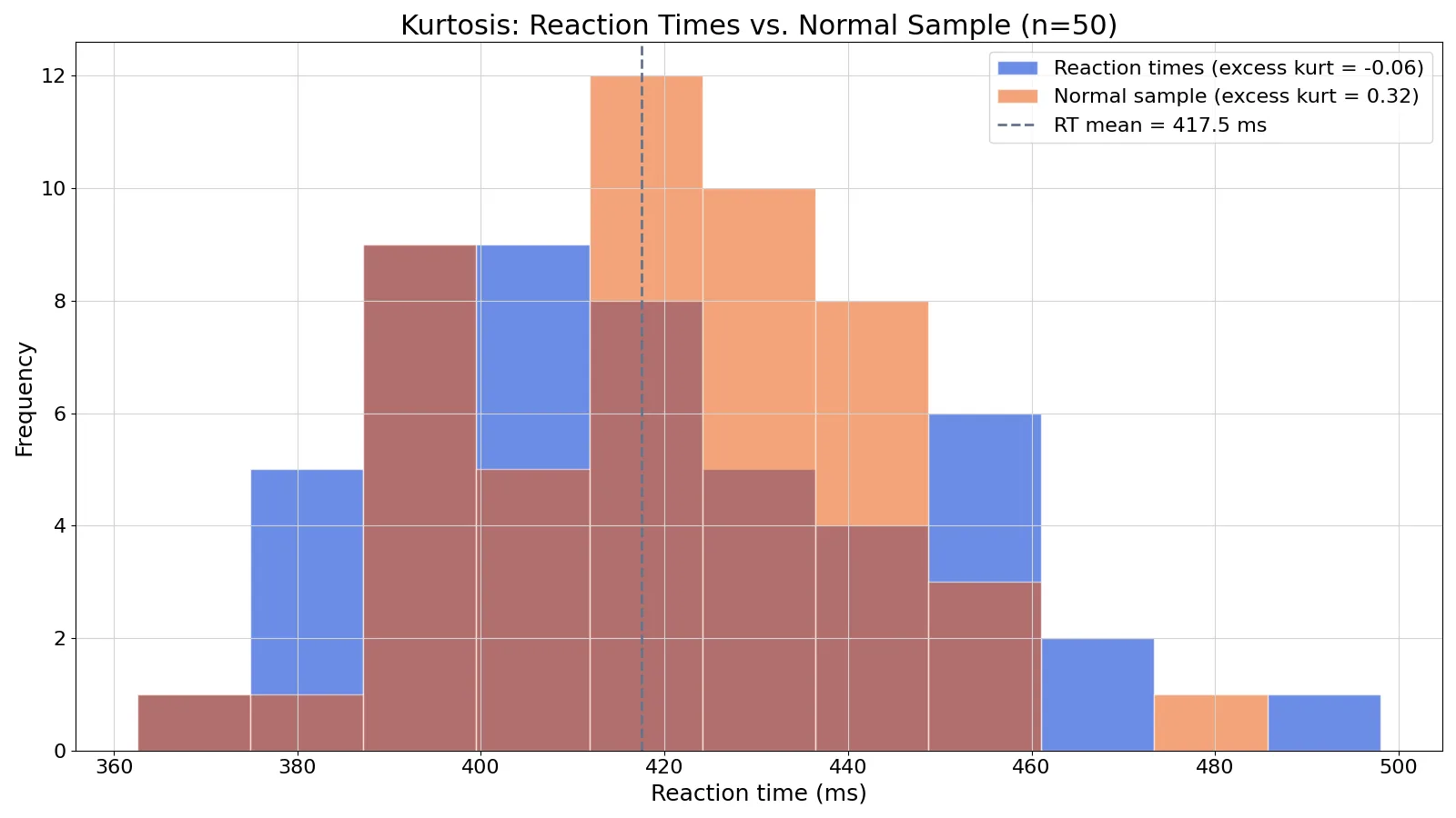
The dataset below contains 50 reaction times in milliseconds from a simple visual reaction-time task.

Reaction time (ms)
412, 388, 455, 401, 372, 498, 421, 390, 410, 433
405, 377, 462, 419, 395, 441, 408, 386, 425, 452
399, 414, 437, 381, 468, 403, 392, 429, 446, 411
375, 458, 417, 397, 435, 406, 383, 449, 423, 394
461, 409, 388, 442, 415, 400, 428, 391, 454, 418

The steps are:

Sample size $n$ = 50
Mean reaction time = 417.4600 ms
Sample standard deviation ($n-1$) = 28.1354 ms
Second moment $m_2$ = 775.7684
Fourth moment $m_4$ = 1,702,844.3371
$m_2^2$ (the divide-by-$n$ SD to the fourth power) = 601,816.6104
Excess kurtosis $g_2 = m_4 / m_2^2 - 3$ = -0.1705
Software excess kurtosis (bias-corrected) = -0.0585
Pearson kurtosis = excess + 3 = 2.9415

For comparison, a normal sample of the same size produced an excess kurtosis of 0.3226 and a Pearson kurtosis of 3.3226.

import numpy as np
from scipy import stats
rt = [...]  # 50 reaction times
excess = stats.kurtosis(rt, fisher=True, bias=False)
pearson = excess + 3
print(f"excess kurtosis = {excess:.4f}; Pearson kurtosis = {pearson:.4f}")

Output:

excess kurtosis = -0.0585; Pearson kurtosis = 2.9415

The reaction times have a slightly negative excess kurtosis, which means their tails are a little lighter than a normal distribution. The value is close to zero, so the distribution is close to mesokurtic.

How to Interpret It

Start by checking whether the reported value is raw kurtosis or excess kurtosis. If a normal distribution should score 3 in your output, you are looking at raw kurtosis. If it should score 0, you are looking at excess kurtosis [2][3].

Then read the sign and size:

Excess kurtosis	Type	Tail behavior
Near 0	Mesokurtic	Tails similar to a normal distribution
Positive	Leptokurtic	Heavier tails, more outliers
Negative	Platykurtic	Lighter tails, fewer outliers

A leptokurtic distribution produces extreme values more often than a normal distribution would. A platykurtic distribution produces them less often, and a uniform distribution, which has no tails at all, is a common example [2][4].

The magnitude depends on your sample size and your field. In small samples, kurtosis estimates bounce around a lot, so a value like -0.06 or 0.32 is not meaningfully different from zero. Treat kurtosis as one signal among several when you assess distribution shape.

When to Use It (and when not to)

Use kurtosis when you want to describe how outlier-prone a variable is, when you are checking distributional assumptions before a parametric test, or when you are comparing the tail behavior of two or more groups [3]. It pairs naturally with skewness, which describes asymmetry, and with histograms and quantile-quantile plots that show shape directly.

Do not use kurtosis as a measure of peakedness. The idea that kurtosis describes how pointy a peak is has been shown to be incorrect, and the central region of a distribution usually contributes very little to the kurtosis value [1]. Do not rely on kurtosis alone to decide whether data are normal, especially in small samples. Do not compare kurtosis values across software packages without confirming that both use the same formula [5].

Kurtosis vs Skewness

Skewness and kurtosis are both shape statistics, but they answer different questions.

Feature	Kurtosis	Skewness
What it measures	Tail heaviness and outlier tendency	Asymmetry of the distribution
Normal distribution value	3 (raw) or 0 (excess)	0
Positive value means	Heavier tails than normal	Longer right tail
Negative value means	Lighter tails than normal	Longer left tail
Power of deviations used	Fourth power	Third power

Skewness tells you whether one side of the distribution stretches further than the other. Kurtosis tells you whether the extremes on both sides are heavier or lighter than a normal distribution [2][4]. You usually report them together.

Common Mistakes

Treating kurtosis as peakedness. The fix is to read it as tail behavior only, since the peak shape is largely unrelated to the kurtosis value [1].
Forgetting the excess adjustment. The fix is to check whether your software subtracts 3, because a value of 3 and a value of 0 can describe the same distribution [2][5].
Comparing values across packages without checking formulas. The fix is to confirm which estimator each package uses before you compare [5].
Judging normality from kurtosis alone. The fix is to combine kurtosis with skewness, plots, and formal tests [3].
Overinterpreting small values in small samples. The fix is to treat values near zero as normal-like unless the sample is large.
Assuming high kurtosis means a tall peak. The fix is to remember that a distribution with a given kurtosis can have a tall, flat or any other peak shape, because kurtosis is driven by the tails [1].

Limitations

Kurtosis is a single number, so it compresses a lot of shape information into one value. Two distributions with the same kurtosis can look very different, and kurtosis says nothing about where the tails bend or how many modes a distribution has. It also cannot tell you whether a specific extreme value is an error or a genuine observation.

Sample kurtosis is sensitive to sample size and to individual extreme points. In small samples the estimate is unstable, and one unusual value can shift it noticeably. Software differences in the formula add another layer of uncertainty, so always report which convention you used [2][5].

Frequently Asked Questions

What is a good kurtosis value?

There is no single good value. For a normal distribution, raw kurtosis is 3 and excess kurtosis is 0. Values close to those benchmarks suggest normal-like tails. What counts as close depends on your sample size and field, so treat any threshold as a general guideline [3].

What does a kurtosis of 3 mean?

A kurtosis of 3 usually means you are looking at raw, or Pearson, kurtosis and the distribution has tails similar to a normal distribution. If your software reports excess kurtosis, the equivalent value is 0. Always confirm which scale your output uses before interpreting the number [2][5].

Is high kurtosis good or bad?

Neither by itself. High kurtosis means the distribution is outlier-prone, which can be a problem for methods that assume normality. In some settings, such as finance, heavy tails are expected and important to model. The meaning depends on your analysis goals [1].

Can kurtosis be negative?

Raw kurtosis cannot be negative because it is built from fourth powers, which are always non-negative. Excess kurtosis can be negative, and it means the distribution has lighter tails than a normal distribution. A uniform distribution has an excess kurtosis of -1.2, and the smallest possible value, -2, occurs for a symmetric two-point distribution [2][4].

Does kurtosis measure the peak of a distribution?

No. Kurtosis measures tail extremity, meaning either the outliers present in a sample or the tendency of a distribution to produce them. The proportion of kurtosis determined by the central region around the mean is usually quite small, so peak shape is not what the statistic captures [1].