Stationarity Definition: What It Means in Time Series

By Dr. Zubair Khalid, DVM, MS, PhD · 2026-10-03

The stationarity definition in time series is simple: a series is stationary when its statistical properties, such as mean, variance and autocorrelation, stay constant over time [1][2]. Most forecasting and regression models on time series assume this property, so checking it is one of the first steps in any analysis. This article explains the definition, the math behind it, and how to test for it with real numbers.

Quick Answer

A stationary series has a constant mean, constant variance and an autocorrelation structure that does not change over time [1].
It looks flat: no trend, no growing or shrinking spread, no repeating seasonal swings [1].
Weak (covariance) stationarity only requires the first two moments to be stable, which is what most models actually need [3].
You check it with rolling means and rolling standard deviations, plus a formal test such as the augmented Dickey-Fuller (ADF) test.
If a series is not stationary, you can difference it, take logs or square roots, or fit and remove a trend [1][2].

What Stationarity Means

In plain terms, a stationary process is one whose behavior does not depend on when you look at it. If you took a window of 12 months from the start of the series and a window of 12 months from the end, the two windows would have roughly the same average level, the same spread, and the same pattern of how each value relates to the previous one [1].

The precise statistical definition comes in two versions. A process $(X_t : t \in T)$ is strictly stationary if the joint distribution of any set of observations is unchanged when you shift all the time points by the same amount $h$ [3]:

$$P(X_{t_1} \leq x_1, \ldots, X_{t_n} \leq x_n) = P(X_{t_1+h} \leq x_1, \ldots, X_{t_n+h} \leq x_n)$$

That condition is hard to verify in practice because it constrains the entire distribution, and too many parameters would have to be estimated from limited data [3]. So analysts usually work with weak stationarity, also called covariance or wide-sense stationarity. A process is weakly stationary when the second moments are finite, $E[X_t^2] < \infty$ for all $t$, the mean is constant, and the autocovariance depends only on the lag between two points, not on their absolute position in time [3][4].

Strict stationarity does not imply weak stationarity unless the relevant moments exist, and the terminology for intermediate forms varies between authors [4]. For everyday modeling, weak stationarity is the working definition.

How It Works

Weak stationarity imposes three conditions on the process. Writing them out makes the mechanism clear:

$$E[X_t] = \mu \quad \text{for all } t$$

$$\text{Var}(X_t) = \sigma^2 \quad \text{for all } t$$

$$\text{Cov}(X_t, X_{t+h}) = \gamma(h) \quad \text{for all } t$$

Each symbol means the following. $X_t$ is the value of the series at time $t$. $\mu$ is the constant mean, the same at every point. $\sigma^2$ is the constant variance, so the spread does not widen or narrow. $\gamma(h)$ is the autocovariance at lag $h$, a function of the gap between two observations only. If you shift both observations forward by any amount, $\gamma(h)$ does not change.

The practical consequence is that a stationary series is predictable in a specific sense. You predict that its statistical properties in the future will match what they were in the past [2]. When a series fails these conditions, you transform it until it passes, then model the transformed version and reverse the transformation to get forecasts on the original scale [2].

Worked Example

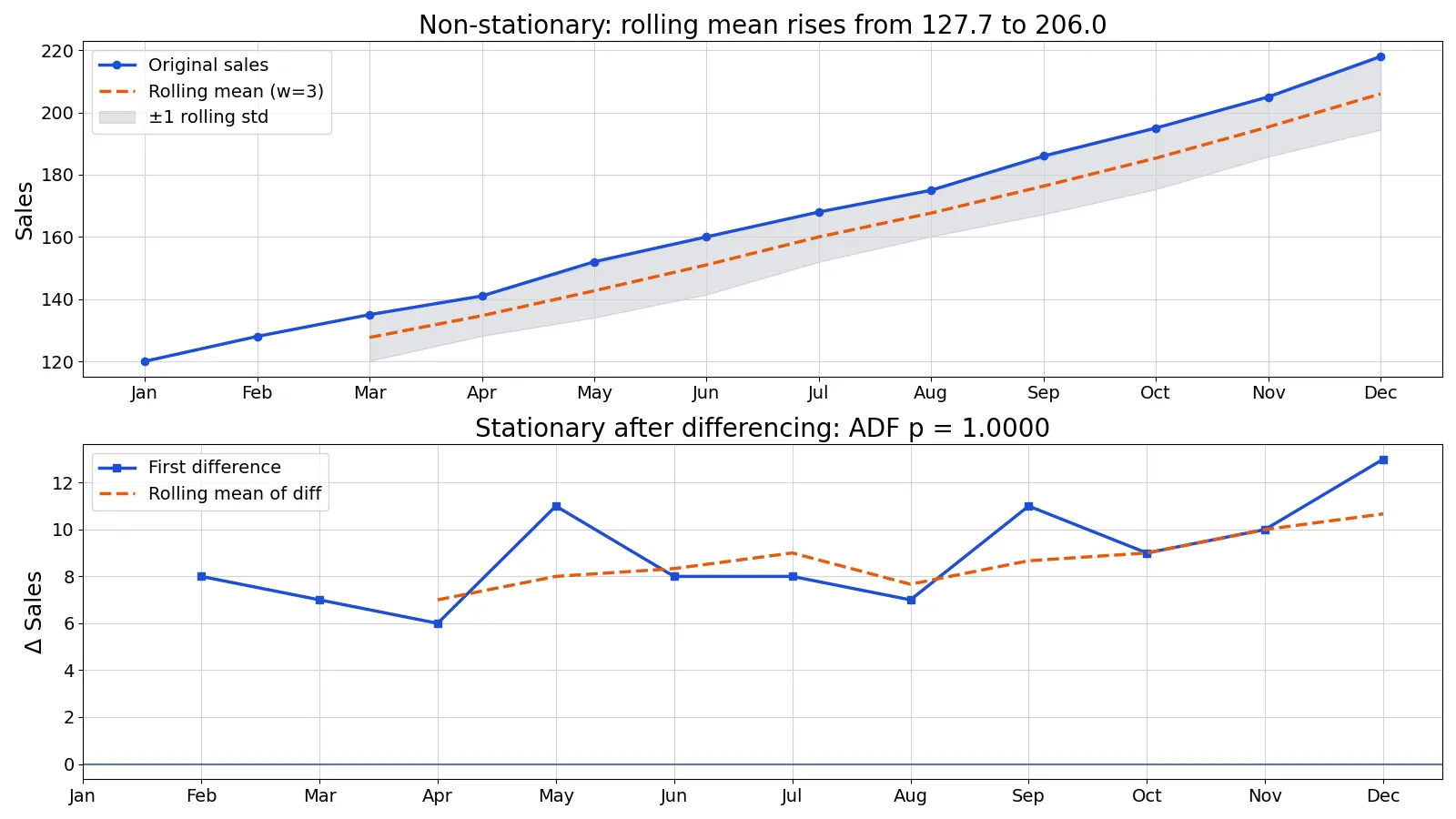
The dataset is monthly sales for one product over 12 months, and it clearly trends upward.

Month	Jan	Feb	Mar	Apr	May	Jun	Jul	Aug	Sep	Oct	Nov	Dec
Sales	120	128	135	141	152	160	168	175	186	195	205	218

A rolling window of 3 months shows whether the level and spread are stable. At March, the rolling mean is $(120 + 128 + 135) / 3 = 127.6667$ and the rolling standard deviation with $ddof=1$ is $\sqrt{((120-127.6667)^2 + (128-127.6667)^2 + (135-127.6667)^2)/2} = 7.5056$. At December, the rolling mean is $(195 + 205 + 218) / 3 = 206.0000$ and the rolling standard deviation is $11.5326$.

Both statistics drift. The mean rises from 127.6667 to 206.0000 and the spread widens from 7.5056 to 11.5326, so the series fails the constant-mean and constant-variance conditions.

The first difference removes the trend. At February, $128 - 120 = 8.0000$. At December, $218 - 205 = 13.0000$. The differenced series has one fewer point than the original [1].

The ADF test confirms the visual read. On the original series the ADF statistic is -1.5857 with a p-value of 0.4908, so you fail to reject the null of a unit root and treat the series as non-stationary. On the first difference the ADF statistic is 3.1059 with a p-value of 1.0000.

import pandas as pd
from statsmodels.tsa.stattools import adfuller
sales = pd.Series([120,128,135,141,152,160,168,175,186,195,205,218])
roll_mean = sales.rolling(3).mean()
roll_std  = sales.rolling(3).std()
diff = sales.diff()
print(f"ADF p-value original = {adfuller(sales)[1]:.4f} (fail to reject -> non-stationary)")
print(f"ADF p-value differenced = {adfuller(diff.dropna())[1]:.4f} (fail to reject -> no evidence of stationarity)")

Output:

ADF p-value original = 0.4908 (fail to reject -> non-stationary)
ADF p-value differenced = 1.0000 (fail to reject -> no evidence of stationarity)

Neither ADF result rejects the unit-root null here, and the differenced p-value of 1.0000 is the one to be careful with. With only 11 differenced observations, the test has almost no power, and a p-value near 1 is not evidence of stationarity. The rolling statistics and the plot are the more trustworthy signal on a sample this small.

How to Interpret It

Read the rolling mean and rolling standard deviation first. A rolling mean that climbs or falls steadily indicates a trend, which breaks the constant-mean condition. A rolling standard deviation that grows indicates changing spread, which breaks the constant-variance condition. A repeating pattern at a fixed interval indicates seasonality, which also violates stationarity and is usually handled by including seasonal terms in the model instead of differencing it away [1].

Then read the ADF p-value as a supporting check. A small p-value is evidence against a unit root, which supports stationarity. A large p-value means you cannot rule out a unit root. Treat the test as one input, not a verdict, especially on short series.

Finally, look at the autocorrelation function. For a stationary series it decays toward zero as the lag grows. A slow, near-linear decay is a common sign of non-stationarity.

When to Use It (and when not to)

Use stationarity as a precondition when you fit models that assume stable moments. ARMA and ARIMA models, most exponential smoothing variants, and regression on time series all rely on it in some form [1][2]. If you are forecasting, the assumption that the future resembles the past is exactly the stationarity assumption, so it pays to check.

Do not force stationarity when the trend itself is the object of interest. If you are measuring growth rates, estimating a trend line, or testing whether a policy changed the level of a series, differencing destroys the signal you want. Do not difference a series that is already stationary, since overdifferencing introduces artificial negative autocorrelation. Do not apply differencing to seasonal data without also handling the seasonal lag.

Stationarity vs White Noise

White noise is a special case of stationarity, and the distinction trips people up.

Property	Stationary series	White noise
Constant mean	Yes	Yes, usually zero
Constant variance	Yes	Yes
Autocovariance at lag 0	Positive	Positive
Autocovariance at lags above 0	Can be nonzero, decays with lag	Zero at every lag above 0
Predictable from its own past	Yes, often	No

Every white noise process is stationary, but most stationary processes are not white noise. A stationary AR(1) process with a positive coefficient has autocorrelation that decays gradually, which makes it forecastable. White noise has no such structure.

Common Mistakes

Judging stationarity from the raw plot alone. A series can look flat while its variance changes. Always compute rolling mean and rolling standard deviation, not just the level.
Treating a large ADF p-value as proof of non-stationarity. The test has low power on short series. Combine it with rolling statistics and the autocorrelation function.
Differencing a series that is already stationary. This introduces negative autocorrelation and makes the model harder to interpret. Check first, then difference.
Ignoring seasonality because the trend is gone. Removing a trend does not remove a repeating seasonal pattern. Handle seasonality explicitly in the model [1].
Applying a log or square root transform to negative values. Add a constant to make all values positive before transforming, then subtract it back when you invert the model [1].
Assuming strict stationarity is required. Most models only need weak stationarity, so the full distributional condition is usually more than you need [3].

Limitations

Stationarity is a property of the data-generating process, and you never observe that process. You observe one realization, so every test is an inference from a single path. Short series make this worse, since both rolling statistics and unit root tests need enough observations to be informative. A p-value near 1 on a differenced series of 11 points, as in the example above, tells you almost nothing.

The definition also says nothing about which transformation is correct. Differencing, logging, detrending and seasonal adjustment all produce different series, and the choice changes your forecasts. Stationarity is a precondition for a model, not a guarantee that the model is right. A stationary series can still be badly forecast by a misspecified model.

Frequently Asked Questions

What is the simple stationarity definition?

A stationary time series is one whose statistical properties, including mean, variance and autocorrelation, do not change over time [1][2]. Practically, it looks flat with no trend, no changing spread and no periodic fluctuations. If those properties shift as time passes, the series is non-stationary.

What is the difference between strict and weak stationarity?

Strict stationarity requires the entire joint distribution to be invariant under time shifts [3]. Weak stationarity only requires finite second moments, a constant mean, and an autocovariance that depends on lag alone [3][4]. Weak stationarity is easier to check and is what most models assume.

How do I test whether my series is stationary?

Start with rolling means and rolling standard deviations over a window you choose. Then run an augmented Dickey-Fuller test and read the p-value. Finally, inspect the autocorrelation function for slow decay. Use all three together, since each has blind spots on short series.

Does differencing always make a series stationary?

No. One difference usually removes a linear trend, and a single difference is often sufficient [1]. But if the series has a seasonal pattern or a changing variance, differencing alone will not fix it. You may need a seasonal difference, a log transform, or both.

Can a series be stationary but still hard to forecast?

Yes. White noise is stationary and completely unpredictable from its own past. Stationarity makes the statistical properties stable, which is necessary for many models, but it does not create predictable structure where none exists.

References

6.4.4.2. Stationarity
Stationarity and differencing of time series data
1.2: Stationary Time Series - Statistics LibreTexts/1%3A_Basic_Concepts_in_Time_Series/1.2%3A_Stationary_Time_Series)
Stationary process - Wikipedia