Normal Distribution Calculators for Life Scientists
By Dr. Zubair Khalid, DVM, MS, PhD ·

By the end of this guide you will be able to take a bell-shaped set of measurements, find the probability of a result above or below any cutoff, work backward from a probability to the cutoff that produces it, and build a 95 percent reference range. You will run the same calculation in R, in Python, in Excel, and in a free web applet, and you will know how to recognize the datasets where the normal model breaks down.
A normal distribution calculator for biology data answers one question in two directions. Given a value, it returns the probability of seeing that value or something more extreme. Given a probability, it returns the boundary value that marks it. That single calculation sits underneath reference ranges, plate quality control limits, outlier rules, and confidence intervals, and it appears inside published methods from disease surveillance to diagnostic marker studies. Normal distribution calculators for life scientists are not a specialty product. The same pnorm function a biostatistician runs is free inside R on any lab laptop, and educators have shown that people without a statistics background can learn these tools when instruction is built around real cases [1].
Here is what to have on hand. Bring a dataset, or just its mean and standard deviation. Bring one tool: R (free from CRAN), Python with SciPy (installed with pip install scipy), Excel or Google Sheets, or any web applet found by searching for a normal distribution calculator. Nothing else is required.
What the Normal Distribution Means in Biology
The normal distribution is a continuous, symmetric, bell-shaped probability curve described completely by two numbers. The mean (μ) locates the center. The standard deviation (σ) sets the spread. Move one standard deviation to either side and you enclose about 68 percent of the values. Two standard deviations enclose about 95 percent. Three enclose about 99.7 percent. This 68-95-99.7 rule is the fastest sanity check you own whenever a calculator hands you an answer.
The z-score standardizes any value:
z = (x - μ) / σ
A z-score of 2 says the value sits two standard deviations above the mean. Because the probability of exceeding a given z is identical for every normal distribution, one calculator serves enzyme activities in U/L, optical densities, cell counts, and body lengths in millimeters without any unit conversion.
Biology leans on this model for two reasons. Many measurements cluster symmetrically around a center, especially replicate measurement error and physiological values within a defined healthy cohort. The intuition is that measurement error is the sum of many small independent influences, and sums of independent influences tend toward the bell shape. The central limit theorem makes this precise: means of sufficiently large samples follow an approximately normal distribution even when the raw data do not, which is why t-tests, ANOVA, and confidence intervals inherit normal-style arithmetic.
The caution comes before the calculation. Cell counts, infection proportions, cytokine concentrations, and incubation periods are usually skewed rather than bell shaped. "Approximately normal" is a working description of your data, not a law of biology. The calculator is a model, and every model earns trust through a fit check, which is Step 1 of the walkthrough below.
Choosing a Normal Distribution Calculator for Biology Work
Four tool families cover every situation in a life science lab.
A web applet is the fastest start. Search for a normal distribution calculator, enter a mean, an SD, and a cutoff, and read the shaded area. These suit homework and one-off checks, though they leave no record behind for a lab notebook.
Excel or Google Sheets already sit open at most benches. The functions NORM.DIST, NORM.INV, and STANDARDIZE cover the three core questions, and the workbook itself becomes the record. Older Excel versions use the legacy names NORMDIST and NORMINV, which compute the same quantities.
R and Python form the reproducible tier, and they double as the bioinformatics calculator tier, because the same one-line functions scale from a single value to a transcriptome-wide matrix with no menus. R is free, and a teaching case study for healthcare graduate students and community researchers successfully piloted it with nine non-statisticians as a complement to the more traditional SPSS [1]. If your lab already licenses SPSS, JMP, or GraphPad Prism, the same math runs behind their dialogs. R also offers dnorm for drawing the curve and rnorm for simulating random normal data, which are handy for teaching and for testing an analysis pipeline before real data arrive.
A general biology calculator, the kind that solves Hardy-Weinberg ratios or dilution series, answers different questions. The normal distribution module is the statistics member of that calculator family, and the table below collects its core formulas in one place.
| Task | Formula | R | Python (SciPy) | Excel / Google Sheets |
|---|---|---|---|---|
| Probability below a cutoff | P(X ≤ x) | pnorm(x, mu, sigma) | norm.cdf(x, loc, scale) | =NORM.DIST(x, mu, sigma, TRUE) |
| Probability above a cutoff | 1 - P(X ≤ x) | 1 - pnorm(x, mu, sigma) | 1 - norm.cdf(x, loc, scale) | =1-NORM.DIST(x, mu, sigma, TRUE) |
| Standardized z-score | z = (x - μ) / σ | (x - mu) / sigma | (x - loc) / scale | =STANDARDIZE(x, mu, sigma) |
| Cutoff for tail probability p | x = μ + zσ | qnorm(p, mu, sigma) | norm.ppf(p, loc, scale) | =NORM.INV(p, mu, sigma) |
| Central 95 percent interval | μ ± 1.96σ | qnorm(c(0.025, 0.975), mu, sigma) | norm.ppf([0.025, 0.975], loc, scale) | =NORM.INV(0.025, ...) and =NORM.INV(0.975, ...) |
| Curve height at x (density) | bell curve height | dnorm(x, mu, sigma) | norm.pdf(x, loc, scale) | =NORM.DIST(x, mu, sigma, FALSE) |
Choose the tool you will reuse. A saved script or workbook answers a reviewer's question years later, and analysts hired into life science roles are expected to produce exactly that kind of record.
Using a Normal Distribution Calculator for Biology Data, Step by Step
The walkthrough uses one running example. You measure an enzyme activity in plasma from 200 healthy adult volunteers. The mean is 50 U/L, the standard deviation is 5 U/L, and the histogram is symmetric and bell shaped. Three questions follow. What proportion of values fall at or below 60 U/L? What cutoff marks the top 5 percent? What range covers the central 95 percent?
Step 1: Fix the Two Parameters and Check the Shape
Store the two parameters, then look at the data before trusting the model. Here activity is your vector of 200 measurements.
mu <- mean(activity)     # 50 U/L in this example
sigma <- sd(activity)    # 5 U/L in this example

hist(activity)           # bell shape?
qqnorm(activity)         # do points hug the line?
qqline(activity)
shapiro.test(activity)   # formal normality test
The Shapiro-Wilk test prints a W statistic between 0 and 1 together with a p-value. A W near 1 with a p-value above 0.05 is consistent with normality. The Q-Q plot, a quantile-quantile plot that graphs your sorted data against the values a normal fit would predict, should hug the straight line. With very large samples the test flags trivial departures, so treat the plot as the primary evidence and the p-value as supporting detail.
Step 2: Convert the Cutoff to a z-Score
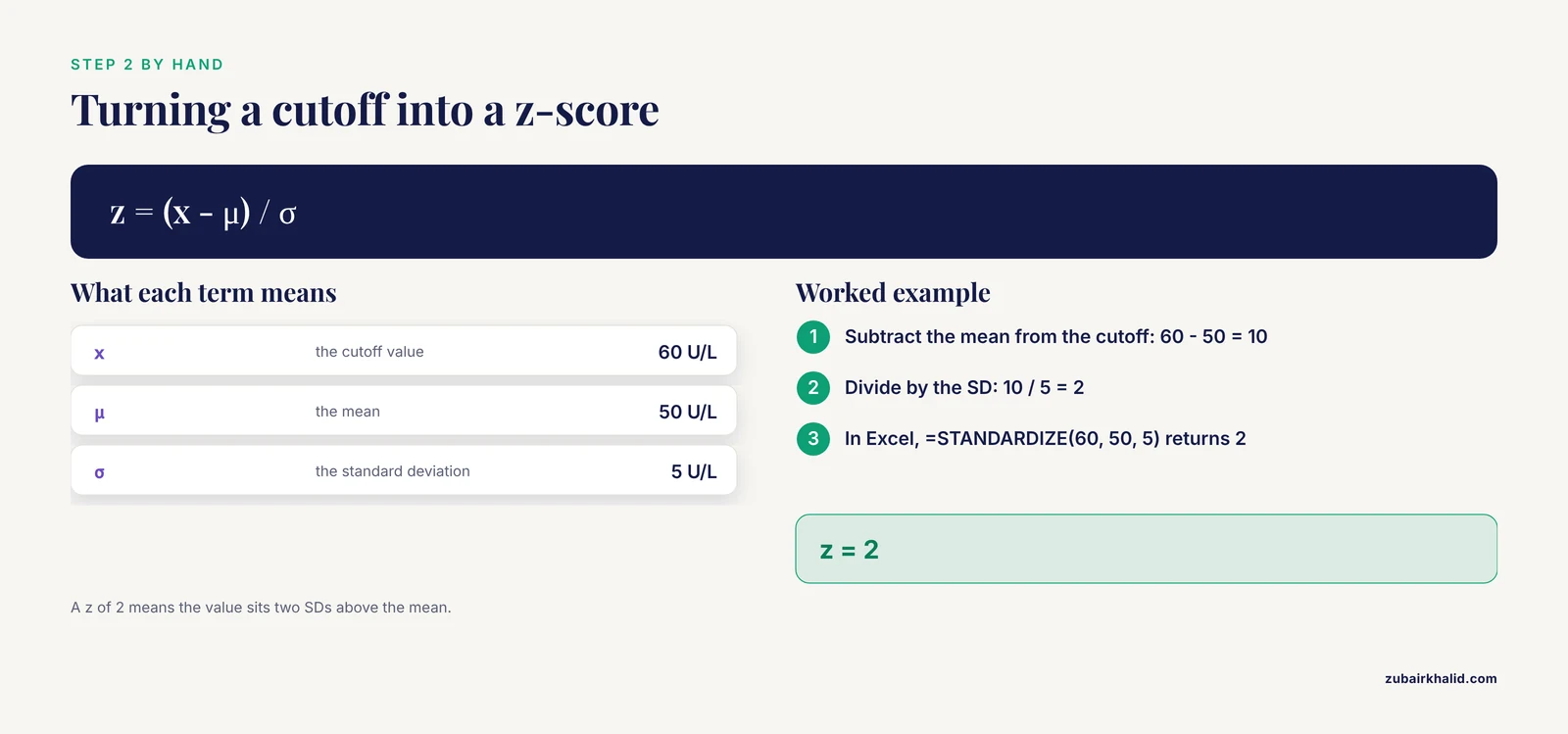
z = (60 - 50) / 5 = 2. The value 60 U/L sits two standard deviations above the mean. In Excel, =STANDARDIZE(60, 50, 5) returns 2. Do this by hand even when the software will do it for you, because every later answer inherits any mistake made here.
Step 3: Convert the z-Score to a Probability
R answers first:
pnorm(60, mean = mu, sd = sigma)
#> [1] 0.9772499

1 - pnorm(60, mean = mu, sd = sigma)
#> [1] 0.02275013
Read this as 97.72 percent of values at or below 60 U/L and 2.28 percent above.
Python returns identical numbers:
from scipy import stats

stats.norm.cdf(60, 50, 5)
# 0.9772498680518208

1 - stats.norm.cdf(60, 50, 5)
# 0.02275013194817921
Excel or Google Sheets:
=NORM.DIST(60, 50, 5, TRUE)
0.977249868

=1-NORM.DIST(60, 50, 5, TRUE)
0.022750132
The TRUE argument requests the cumulative area to the left of the cutoff, the quantity statisticians call the cumulative distribution function, or CDF. FALSE returns the height of the bell curve at that point, the probability density, which is for drawing the curve and never for probabilities.
Step 4: Work Backward With the Inverse Calculator
To flag the highest 5 percent of results, ask for the 95th percentile, the value that leaves 95 percent of the area to its left. Functions named for quantiles (qnorm, NORM.INV, norm.ppf) invert the CDF.
qnorm(0.95, mean = mu, sd = sigma)
#> [1] 58.22427
Python: stats.norm.ppf(0.95, 50, 5) returns 58.22426813475736. Excel: =NORM.INV(0.95, 50, 5) returns 58.22426813. Any result above roughly 58.2 U/L lands in the top 5 percent under this model.
Step 5: Build the Central 95 Percent Range and Check It
qnorm(c(0.025, 0.975), mean = mu, sd = sigma)
#> [1] 40.20018 59.79982
This is the classic mean ± 1.96 SD reference range, here 40.2 to 59.8 U/L, the interval expected to contain 95 percent of individual values from the same population.
Two checks confirm the machinery. First, 60 U/L is exactly two SDs above the mean, and the 68-95-99.7 rule predicts roughly 2.5 percent above it, close to the exact 2.28 percent. Second, symmetry: the probability below 40 U/L must equal the probability above 60 U/L.
pnorm(40, mean = mu, sd = sigma)
#> [1] 0.02275013
The tails match. When they do not, a variance went into an SD box or a tail got flipped.
Exact Error Messages and Fast Fixes
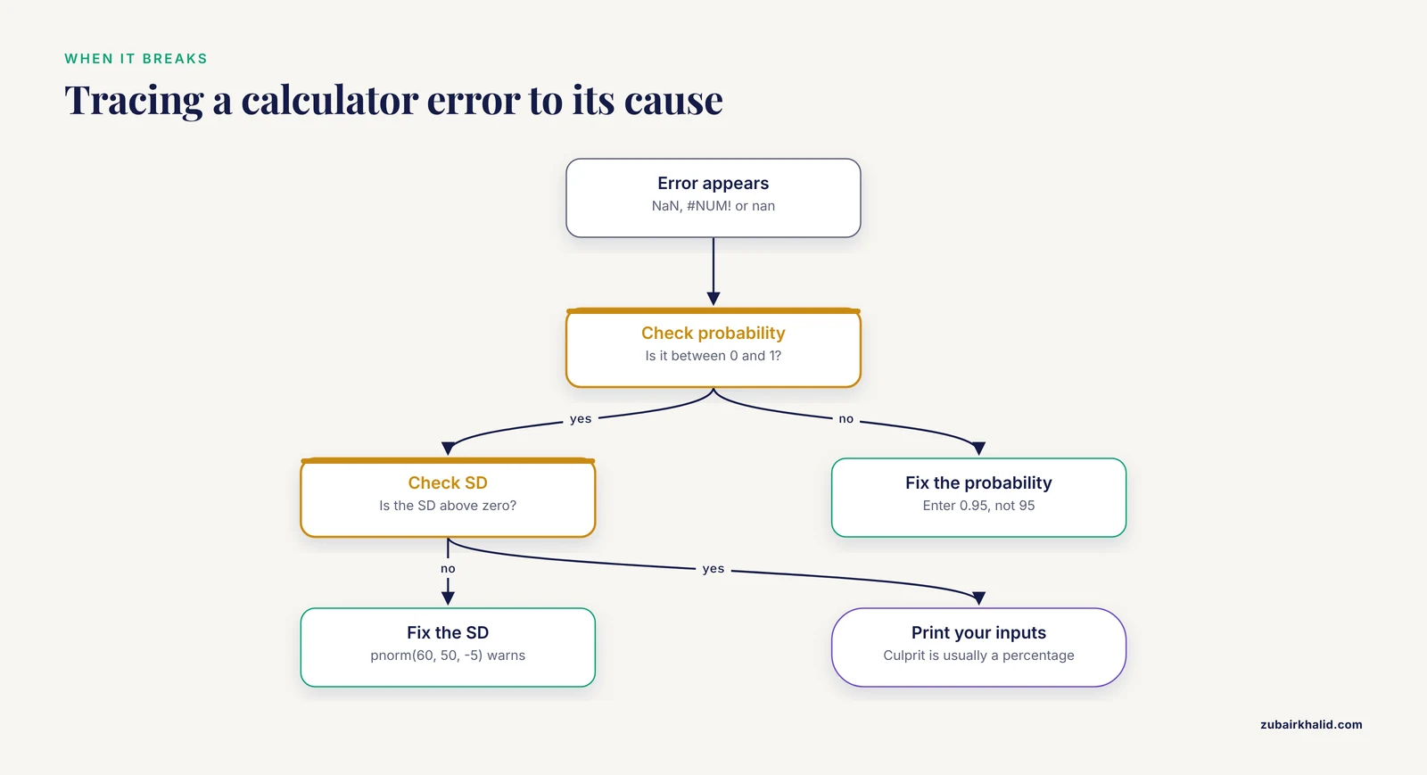
Three messages cover most calculator failures.
R prints NaN with a warning when a probability leaves the legal range:
qnorm(1.5)
#> [1] NaN
#> Warning message:
#> In qnorm(1.5) : NaNs produced
The fix is to feed qnorm a probability between 0 and 1, and to feed every function a positive SD. pnorm(60, 50, -5) produces the same warning.
Excel returns #NUM! for the same two causes. =NORM.INV(1.5, 0, 1) and =NORM.DIST(60, 50, 0, TRUE) both return #NUM!. Check that the probability lies between 0 and 1 and that the SD is greater than zero.
SciPy returns nan for out-of-range probabilities, sometimes with a RuntimeWarning. Print your inputs when nan appears, because the culprit is almost always a percentage entered as 95 instead of 0.95.
Worked Examples From Biology Labs and Public Health
Example 1: a plate QC limit. Your blank wells read a mean optical density of 0.85 with an SD of 0.12 at 450 nm. How often would a blank cross 1.0 by chance alone?
1 - pnorm(1.0, mean = 0.85, sd = 0.12)
#> [1] 0.1056498
About 10.6 percent of blanks would trip that flag through luck, so the limit sits too close to the blank distribution. Raise the limit or investigate the drift before chasing phantom contamination.
Example 2: a published surveillance method. Geographic cluster detection asks which areas hold more disease events than chance explains. Torabi and Rosychuk proposed detecting clusters of disease-related events with an approximate normal distribution, replacing a compound Poisson calculation (a model for counts of random events whose probabilities become cumbersome to compute when events are numerous or analyses are split by strata). They showed the normal approach is very easy to implement when population sizes are large and demonstrated it on pediatric self-inflicted injury presentations to emergency departments [2]. The arithmetic inside that published method is the same pnorm calculation from Step 3.
Example 3: from single values to sample means. If individual activities carry an SD of 5 U/L, the mean of 25 independent samples carries a standard error of 5 / √25 = 1 U/L. The standard error is the SD of the sample mean, and it shrinks as sample size grows. A 95 percent confidence interval for a mean of 50 U/L is therefore 50 ± 1.96 × 1, which is 48.0 to 52.0 U/L. When the SD itself was estimated from a small sample, swap the normal multiplier for a t multiplier, a distinction the mistakes section takes up.
Normal Distribution Calculator Tips for Biology Data
- Decide the tail before you type. Write down whether you want the area below, above, or outside a range. Most wrong answers are tail errors, not arithmetic errors.
- Enter the SD, never the variance. Variance is SD squared. A paper that reports a variance of 25 is reporting an SD of 5. The unit test catches this instantly: the SD carries the units of the measurement (U/L), the variance carries squared units.
- Match the question to the function. pnorm answers "what proportion lies below this value." qnorm answers "what value marks this proportion." Mixing them is the most common beginner error in R.
- Keep full precision until the final report. Chain rounded numbers through several steps and the drift appears in the third decimal of your cutoff.
- Practice on your own data. The educators who taught multivariate methods to non-statisticians built lessons around interactive data from the students themselves, and that active approach makes the functions stick [1].
- Transform skewed measurements first. A log10 or natural-log transform often straightens right-skewed biochemical values. Run the calculator on the transformed scale, back-transform the endpoints at the end, and remember that a mean computed on the log scale back-transforms to the geometric mean.
- Use the SD for questions about individuals and the standard error for questions about means. They differ by a factor of √n, and swapping them is how reference ranges come out impossibly narrow.
- Record the tool, function, and version in your methods section or notebook. pnorm in R and NORM.DIST in Excel agree to many decimal places, but a reviewer can only verify what you named.
Common Mistakes and Limitations
Most failures with a normal distribution calculator in biology come from feeding it the wrong data or reading it as something it is not. Each mistake below has a fast fix.
Skipping the fit check. The calculator assumes a bell and never verifies one. Run the histogram, Q-Q plot, and Shapiro-Wilk check from Step 1 before any probability leaves your notebook. With thousands of observations the test flags trivial departures, so read the plot first and treat a tiny p-value on a huge sample as a prompt to look closer, not as a verdict.
Feeding it bimodal data. A distribution with two peaks has a mean that falls in the valley between them, where few real observations live. The Global Burden of Disease 2023 analysis of bone cancers found a bimodal age distribution, with incidence peaking at ages 10 to 14 and rising again in older age groups [3]. A single mean and SD across those ages would describe an age band that barely exists. Plot first, then split the data by whatever separates the peaks, such as age band, genotype, or treatment.
Feeding it bounded, skewed data. Proportions and prevalences cannot fall below 0 or above 1, and survey estimates often scatter far from any center. A meta-analysis of Blastocystis across 562,327 participants found a pooled prevalence of 17.9 percent, with a 95 percent prediction interval (the range where a single new study would likely land) of 0.7 to 87.5 percent, and I² of 99.7 percent, meaning nearly all the variation across studies was real heterogeneity rather than chance [4]. A normal calculator pointed at numbers like those will output a negative prevalence without complaint. Use logit transforms (which map proportions onto an unbounded scale), binomial models, or meta-analytic pooling instead.
Confusing the two meanings of "normal." Statistical normal describes a curve shape. Clinical normal describes a reference label. The BMI literature shows how far apart these are: people with a normal BMI can carry substantial metabolic abnormality, while some people with obesity remain metabolically healthy [5]. A value inside a reference range is not a certificate of health, and a bell curve is not a claim about healthiness. Keep the two vocabularies separate in notes and reports.
Swapping the SD for the standard error. The reference range in Step 5 used the SD of individual values. Substitute the standard error and the range shrinks by a factor of √n, which at n = 25 is a fivefold overstatement of precision.
Using z when the sample is small and σ is unknown. The normal calculator assumes the true SD is known. With fewer than about 30 observations and an SD estimated from the sample, switch to the t-distribution, which has heavier tails to absorb that extra uncertainty:
qt(0.975, df = 24)   # t multiplier for 24 degrees of freedom
#> [1] 2.063899

qnorm(0.975)         # normal multiplier
#> [1] 1.959964
The t multiplier is wider, and that width is honest.
Trusting large samples to fix a bad shape. A large n makes the sample mean approximately normal through the central limit theorem. It does nothing for the raw data. Ten thousand skewed measurements are still skewed, and a reference range computed on them still misrepresents the population.
Reading output as a verdict. The calculator assumes a model, it does not test one, and a probability is not a diagnosis. Decisions about an individual patient or animal belong with a qualified clinician or veterinarian, not with a z-score.
Model limits sit beyond user error. Published summaries arrive rounded, instruments drift, and real distributions carry shoulders the ideal curve lacks. Many modern analyses therefore skip normal-theory cutoffs entirely, which is where the next section picks up.
When Your Data Are Not Normal
You have four honest options.
Transform the variable. A log or square-root transform often makes right-skewed biochemical data symmetric enough for the normal calculator, applied on the transformed scale throughout.
Switch tests. Mann-Whitney, Wilcoxon, and Kruskal-Wallis procedures rank data instead of assuming a shape, and they report medians rather than means.
Resample. Bootstrap and permutation methods build empirical distributions from your own observations, for example by recomputing the mean thousands of times on random draws from your sample, and they need no shape assumption at all.
Model the data type. Counts take Poisson or negative binomial models, proportions take binomial models with a logit link, and that is precisely why large heterogeneous surveys get pooled with random-effects machinery instead of a single bell curve [4].
Diagnostic cutoffs rarely come from mean ± 2 SD anymore. A transcriptomic study of urothelial carcinoma evaluated candidate markers with ROC analysis (receiver operating characteristic, a plot of sensitivity against false-positive rate across every possible cutoff) and machine learning models, reporting areas under the curve (AUC) of 0.927 for IL6ST, 0.921 for LIFR, and 0.843 for JAK1 [6]. AUC runs from 0.5, no better than a coin flip, to 1.0, perfect separation, so those markers distinguish cases from controls well, and their cutoffs were optimized on real diagnostic performance rather than assumed from a curve.
The central limit theorem keeps normal calculators useful even here. Means of enough observations are approximately normal whatever the raw data look like, so confidence intervals for means remain on solid ground. Practical next steps: rerun the walkthrough on one of your own datasets, add a Q-Q plot to your standard analysis script, and read one methods section per week that names its normality check.
Frequently Asked Questions
What is a normal distribution calculator in biology?
A tool that converts a mean, a standard deviation, and a cutoff into the probability of a result beyond that cutoff, or the reverse. In practice that means pnorm or qnorm in R, NORM.DIST or NORM.INV in Excel, norm.cdf or norm.ppf in SciPy, or a shaded web applet.
How do I calculate a z-score for my data step by step?
Subtract the mean from your value and divide by the standard deviation. For a value of 60 with a mean of 50 and an SD of 5, z = (60 - 50) / 5 = 2, and that z feeds straight into the probability side of the calculator.
Which tool should I use, R, Python, Excel, or a website?
All four return the same numbers, so choose by workflow. Websites suit one-off homework, Excel suits bench records, and R or Python suit reproducible scripts and large datasets. R in particular has a manageable learning curve for beginners, as teaching case studies with non-statisticians have shown [1].
How do I check that my data are normal enough?
Look at a histogram and a Q-Q plot, then run a Shapiro-Wilk test. A straight Q-Q line and a p-value above 0.05 support the normal model, and with very large samples the plot deserves more trust than the test.
What is the difference between pnorm and qnorm?
pnorm turns a value into a probability, the cumulative area to its left. qnorm turns a probability into the boundary value. They are inverses of each other, and mixing them up is the most common syntax error.
Can I use a normal calculator on percentages or prevalence data?
Not directly. Proportions are bounded at 0 and 1 and usually skewed, so use a logit transform, a binomial model, or meta-analytic pooling instead.
What does the 68-95-99.7 rule mean at the bench?
About 68 percent of values fall within one SD of the mean, 95 percent within two, and 99.7 percent within three. Use it to eyeball whether a calculator answer is plausible before you trust it.
When should I use something other than a normal distribution calculator?
When data are skewed, bimodal, bounded, or ordinal, or when a cutoff must be optimized for diagnostic performance. ROC analysis and machine learning methods handle those jobs better than a fixed z-score rule [6].
Sources
- Teaching Confirmatory Factor Analysis to Non-Statisticians: A Case Study for Estimating Composite Reliability of Psychometric Instruments.
- Spatial event cluster detection using an approximate normal distribution.
- Global, Regional, and National Burden of Bone Cancers, 1990 to 2023, With Forecasts to 2050: A Systematic Analysis for the Global Burden of Disease Study 2023.
- Blastocystis sp. in human populations: Pooled prevalence and subtype distribution from a systematic review and meta-analysis.
- Metabolic Vulnerability Despite Normal BMI: From Adverse Body Composition to Ectopic Fat and Organ Dysfunction.
- Integrated Transcriptomic and Network Analysis Identifies Diagnostic and Immune-Associated Hub Genes in Urothelial Carcinoma.