Kruskal-Wallis Test: Definition, Formula and Examples

By Dr. Zubair Khalid, DVM, MS, PhD · 2026-10-03

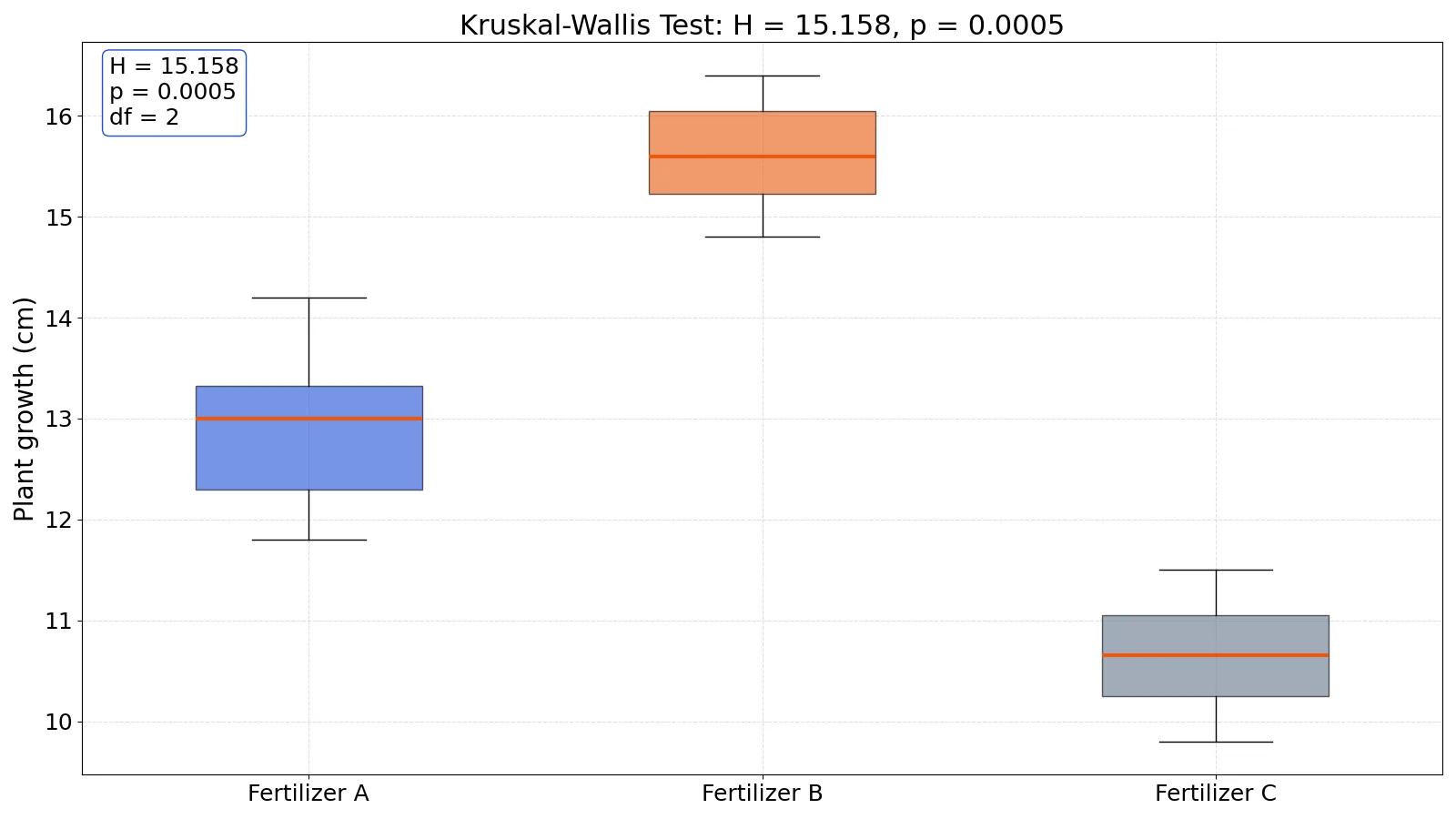
The Kruskal-Wallis test is a non-parametric method for comparing three or more independent groups when your data are not normally distributed or are measured on an ordinal scale. It ranks all observations together, then asks whether the average ranks differ across groups. If the groups really come from the same distribution, the ranks should be mixed fairly evenly.

Quick Answer

The Kruskal-Wallis test compares the medians (more precisely, the central tendency) of two or more independent groups using ranks instead of raw values [1][2].
It is the non-parametric counterpart of one-way ANOVA, so it does not require normally distributed data [3][4].
The test statistic is H, which follows an approximate chi-square distribution with $k - 1$ degrees of freedom, where $k$ is the number of groups [5].
A small p-value means at least one group differs, but the test does not tell you which one. You need post hoc comparisons for that [1].
Each group should have roughly 5 or more observations for the chi-square approximation to work well [3][2].

What the Kruskal-Wallis Test Means

In plain terms, the Kruskal-Wallis test asks a simple question: if you lined up every observation from every group and ranked them from smallest to largest, would one group's values cluster near the top or bottom of that list? If the groups are truly alike, each group should collect a similar share of high and low ranks.

The precise statistical definition is this. The test evaluates the null hypothesis that the population medians of all groups are equal, against the alternative that at least one population median differs [1]. It assumes the variables come from underlying continuous distributions and that the samples are independent [2]. The R documentation describes the null as the location parameters of the distribution being the same in each group [6].

The test was introduced by William Kruskal and W. Allen Wallis in a 1952 paper in the Journal of the American Statistical Association [1].

How It Works

The procedure has three stages: rank, sum, and compare.

First, pool all observations from all groups into one list and assign ranks from 1 (smallest) to $N$ (largest), where $N$ is the total number of observations. Tied values get the average of the ranks they would have occupied [2].

Second, add up the ranks within each group to get $R_i$, the sum of ranks for group $i$.

Third, compute the test statistic:

$$H = \frac{12}{N(N+1)} \sum_{i=1}^{k} \frac{R_i^2}{n_i} - 3(N+1)$$

Each symbol means:

$N$ is the total sample size across all groups.
$k$ is the number of groups being compared.
$n_i$ is the sample size of group $i$.
$R_i$ is the sum of ranks for group $i$.

An equivalent form replaces $R_i^2$ with $n_i \bar{r}_i^2$, where $\bar{r}_i$ is the mean rank in group $i$ [5].

Under the null hypothesis, $H$ follows an approximate chi-square distribution with $k - 1$ degrees of freedom, provided the group sizes are not too small, roughly $n_i > 4$ [2]. You compare $H$ to that distribution to get a p-value. A correction for tied ranks is available and usually changes the result very little [5].

Worked Example

A researcher grows plants under three fertilizer treatments, six plants per treatment, and records growth in centimeters after four weeks. The data are not normally distributed, so a rank-based test fits better than ANOVA.

Fertilizer A	Fertilizer B	Fertilizer C
12.1	15.3	10.2
13.4	16.1	11.5
11.8	14.8	9.8
14.2	15.9	10.9
12.9	16.4	11.1
13.1	15.2	10.4

Step 1: Sample sizes. Each group has $n_i = 6$, so $N = 18$ and $k = 3$.

Step 2: Rank the pooled data and sum by group. Ranking all 18 values together and adding the ranks within each fertilizer gives:

$$R_1 = 57.0, \quad R_2 = 93.0, \quad R_3 = 21.0$$

Fertilizer B collects the highest ranks, Fertilizer C the lowest.

Step 3: Compute H.

$$H = \frac{12}{18 \times 19} \left( \frac{57.0^2}{6} + \frac{93.0^2}{6} + \frac{21.0^2}{6} \right) - 3 \times 19 = 15.1579$$

Step 4: Degrees of freedom. $df = k - 1 = 3 - 1 = 2$.

Step 5: p-value. Comparing $H = 15.1579$ to a chi-square distribution with 2 degrees of freedom gives $p = 0.0005$.

The same result comes out of SciPy:

from scipy.stats import kruskal
A = [12.1, 13.4, 11.8, 14.2, 12.9, 13.1]
B = [15.3, 16.1, 14.8, 15.9, 16.4, 15.2]
C = [10.2, 11.5, 9.8, 10.9, 11.1, 10.4]
H, p = kruskal(A, B, C)
print(round(H, 4), round(p, 4))

Output:

15.1579 0.0005

The group medians were 13.0 cm for Fertilizer A, 15.6 cm for Fertilizer B, and 10.65 cm for Fertilizer C. The group means were 12.9167, 15.6167, and 10.65.

How to Interpret It

The p-value answers one question: how likely is a spread of ranks this uneven if all groups really share the same median? Here $p = 0.0005$, so that is very unlikely. You reject the null hypothesis and conclude that at least one fertilizer produces different growth.

What you cannot conclude is which fertilizer differs. Rejecting the null does not identify the odd group out, and post hoc comparisons between groups are required to find it [1]. A common follow-up is pairwise Mann-Whitney tests with a multiplicity adjustment, or Dunn's test.

It also helps to look at the direction of the effect. The rank sums already hint at it: Fertilizer B has the largest sum of ranks and Fertilizer C the smallest, so the difference likely involves those two. The Kruskal-Wallis test vs. one-way ANOVA guide walks through the follow-up options in more detail.

When to Use It (and when not to)

Use the Kruskal-Wallis test when:

You have three or more independent groups and a continuous or ordinal outcome [5].
The outcome is clearly non-normal, heavily skewed, or has outliers that would distort means.
Your sample is too small to check normality meaningfully [3].
You want a test that depends only on the ordering of values, not their exact spacing.

Do not use it when:

Your groups are paired or matched. Use Friedman's test instead.
You only have two groups. The Mann-Whitney U test (Wilcoxon rank sum) is the two-group case [6].
Your data are genuinely normal and you care about means. One-way ANOVA has more power in that situation [4].
You need to estimate an effect size in the original units. Ranks do not translate back to centimeters or dollars.

Kruskal-Wallis vs One-Way ANOVA

Feature	Kruskal-Wallis	One-Way ANOVA
Data type	Continuous or ordinal	Continuous
Distribution assumption	None required	Normal residuals
Compares	Medians / mean ranks	Means
Test statistic	$H$, chi-square with $k-1$ df	$F$, with two df values
Sensitivity to outliers	Low	High
Power when data are normal	Slightly lower	Higher
Post hoc	Dunn, pairwise Mann-Whitney	Tukey, Bonferroni, Scheffé

The two tests often agree on the conclusion. When they disagree, it usually means the data are skewed or the variances are unequal, and the rank-based result is the safer one [4]. If you are still deciding between parametric options, the two sample t-test guide covers the two-group parametric case.

Common Mistakes

Reporting only the p-value. The test says "some group differs" and nothing more. Always follow a significant result with pairwise comparisons and report which groups differ [1].
Running it on paired data. Kruskal-Wallis requires independent samples. If the same subjects appear in more than one group, use Friedman's test [2].
Treating a non-significant result as proof of equality. Failing to reject the null means you lacked evidence of a difference, not that the medians are identical.
Ignoring tiny groups. With fewer than about 5 observations per group, the chi-square approximation for $H$ is unreliable and you need exact tables [3][2].
Forgetting the tie correction when ties are heavy. Tied ranks are common with ordinal or rounded data, and the correction matters more as ties accumulate [5].
Confusing the median with the mean. The test is about central tendency in ranks. If your groups have equal medians but very different spreads, the test can still flag a difference.

Limitations

The Kruskal-Wallis test is a test of central tendency, not a full comparison of distributions. If two groups have the same median but different shapes or variances, the test can return a significant result that has nothing to do with the median. It also assumes the groups differ only in location when you interpret a significant result as a median difference.

The test gives you no effect size in the original measurement units, and it cannot rank the groups for you. It also loses power relative to ANOVA when the normality assumption actually holds. For small samples, the chi-square p-value is only an approximation, and exact methods are preferable [6][2].

Frequently Asked Questions

What is the difference between the Kruskal-Wallis test and ANOVA?

ANOVA compares group means and assumes normally distributed data with similar variances. Kruskal-Wallis compares group medians using ranks and makes no distributional assumption [3][4]. Use Kruskal-Wallis when normality fails or your data are ordinal.

What does a significant Kruskal-Wallis result tell me?

It tells you that at least one group's median differs from the others. It does not tell you which group, so you must run post hoc pairwise comparisons to locate the difference [1].

How many observations do I need per group?

A common guideline is at least 5 observations per group so the chi-square approximation for $H$ is reasonable [3][2]. With fewer, consult exact critical value tables.

Can I use Kruskal-Wallis with only two groups?

Yes, it works with two groups, but the Mann-Whitney U test is the standard choice for that case and gives you the same essential information [6]. Kruskal-Wallis is designed for three or more groups.

Does Kruskal-Wallis test medians or means?

It tests whether the population medians are equal [1]. Because it works on ranks, it is really testing whether the groups share the same central tendency, and a significant result can also reflect differences in distribution shape.

How do I run it in R?

Use kruskal.test(y ~ group, data = mydata) for a formula interface, or pass a list of numeric vectors directly with kruskal.test(list(g1, g2, g3)) [6]. The output includes the H statistic, degrees of freedom, and p-value.