How to Use a Diagnostic Test Accuracy Calculator for Meta-Analysis

By Dr. Zubair Khalid, DVM, MS, PhD · 2026-11-11

By the end of this guide you will be able to take a set of diagnostic accuracy studies, enter each study's 2 x 2 counts into a diagnostic test accuracy meta-analysis calculator, and walk away with pooled sensitivity, pooled specificity, a summary receiver operating characteristic (SROC) curve, and a defensible heterogeneity assessment. You need a spreadsheet with four counts per study and one of the free tools covered below: the Meta-DiSc 2.0 web application, the MetaDTA package, or R with the mada package.

These tools belong to the same family as any biology calculator you have used, from a Hardy-Weinberg solver to a dilution helper. The difference sits under the hood. A diagnostic test accuracy (DTA) calculator fits a bivariate random-effects model that pools sensitivity and specificity together while tracking how both vary between studies. The payoff is real. A bivariate random-effects analysis of the Biofire FilmArray Meningitis/Encephalitis panel pooled 19 studies and estimated sensitivity of 89.5 percent (95% CI 81.1 to 94.4) and specificity of 97.4 percent (95% CI 94 to 98.9) for detecting bacterial central nervous system infections [1]. This guide shows you, step by step, how to produce estimates of that kind from your own data and how to avoid the errors that sink manuscripts.

What a Diagnostic Test Accuracy Meta-Analysis Calculator Does

Start with the vocabulary, because every field in the calculator maps to one of these terms.

The index test is the test being evaluated, for example a rapid biomarker or an imaging criterion. The reference standard is the best available method that defines who truly has the target condition, for example culture or histopathology. Each primary study cross-classifies its patients into four groups, which form the 2 x 2 table: true positives (TP), false positives (FP), false negatives (FN), and true negatives (TN).

Sensitivity is the proportion of diseased patients the index test correctly flags, TP / (TP + FN). Specificity is the proportion of disease-free patients the test correctly clears, TN / (TN + FP). A DTA meta-analysis pools these two proportions across studies.

The reason a dedicated calculator exists is that sensitivity and specificity are coupled. A study using a lenient cutoff flags more cases, which raises sensitivity while sacrificing specificity, and a strict cutoff does the reverse. Pooling the two proportions separately, as if they were independent, discards that tradeoff and can produce biased, clinically misleading estimates [2]. The bivariate random-effects model solves this by estimating a mean logit sensitivity, a mean logit specificity, the between-study variance of each, and the correlation between the two, all in one model [3]. Schlattmann's tutorial lays out the full methodological ladder: univariate pooling of sensitivity and specificity, univariate random-effects logistic regression, the diagnostic odds ratio, and finally the bivariate model with an exact binomial likelihood for within-study variability, which the tutorial presents as the method of choice [3]. Every credible DTA calculator implements some version of that final model.

If you arrive from machine learning or computational biology, the framing is familiar. This is a bioinformatics calculator problem in miniature, pooling classifier validation counts against a ground truth, and the bivariate model is the statistically honest way to do it.

The Data You Need Before You Start

Every row of your dataset is one primary study, and every row needs four counts. Here is the 2 x 2 table for a single hypothetical study used throughout this walkthrough:

	Disease present	Disease absent
Index test positive	TP = 45	FP = 10
Index test negative	FN = 5	TN = 140

Extract these counts from the results section of each paper. Some studies report sensitivity, specificity, and sample sizes without the full table. In that case you can back-calculate the four cells from the reported proportions and the disease and non-disease counts, and you should flag any row where you had to reconstruct values. Also record, in separate columns, the cutoff or positivity criterion each study used, because thresholds drive the spread you will later see on the SROC plot.

Choosing a Diagnostic Test Accuracy Meta-Analysis Calculator

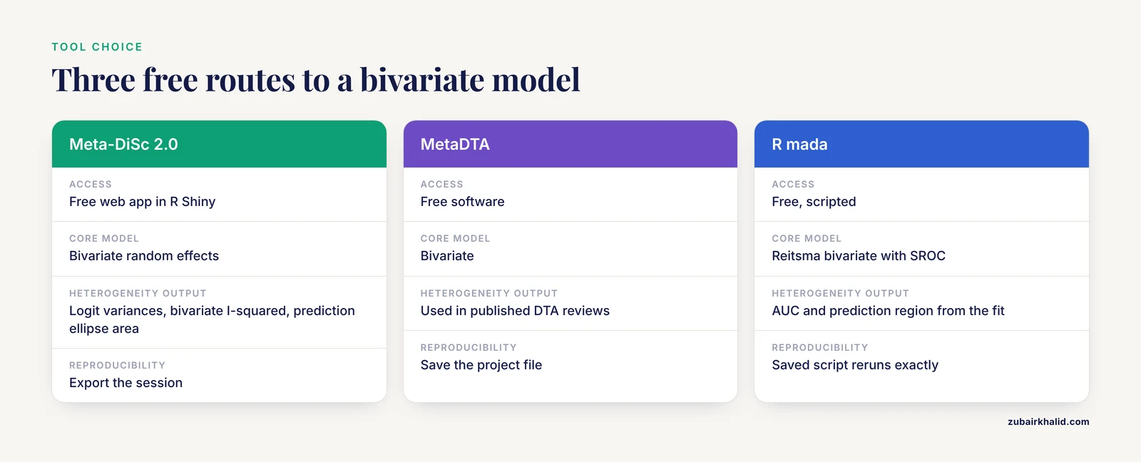
Comparison of Meta-DiSc 2.0, MetaDTA and R with the mada package by access, core model, heterogeneity output and reproducibility.

Three free routes cover almost every need, and a fourth covers Stata users. Meta-DiSc 2.0 is a web application built in R Shiny that implements the bivariate random-effects model and reports a thorough heterogeneity workup, including logit variance estimates, the bivariate I-squared, the area of the 95% prediction ellipse, and median odds ratios for sensitivity and specificity [4]. MetaDTA is the software behind pooled estimates in published DTA reviews such as the analysis of ST-segment elevation for acute coronary occlusion [5]. R gives you scripted, reproducible analyses with the mada package. Stata users can choose among the metandi, midas, and metadta commands, and a recent methods guide compares their strengths and limitations in detail [2].

If your project compares two index tests head to head, the same calculators handle it. A published DTA meta-analysis ran one bivariate hierarchical model per modality to compare endoscopic ultrasound with MRI for rectal cancer staging [6], and a 2024 review used the same framework to compare procalcitonin with C-reactive protein in febrile infants [7].

Tool	Access	Core model	Best fit
Meta-DiSc 2.0	Free web app	Bivariate random effects	Point-and-click runs with a full heterogeneity panel [4]
MetaDTA	Free software	Bivariate	Published DTA reviews use it for pooled estimates [5]
R (mada package)	Free, scripted	Reitsma bivariate, SROC	Reproducible code and custom plots
Stata (metandi, midas, metadta)	Commercial	Hierarchical random effects	Stata workflows with documented commands [2]

Step-by-Step Walkthrough With a Diagnostic Test Accuracy Meta-Analysis Calculator

Step 1: Build the dataset

Create a CSV with one row per study and the four counts in named columns. The mada package expects the column names TP, FP, FN, TN, so use them from the start.

study,TP,FP,FN,TN
A,45,10,5,140
B,30,15,10,95
C,60,8,12,120
D,25,20,8,60
E,38,6,7,99

This five-study set is a teaching dataset. Replace the counts with your own extracted values and keep the same structure.

Step 2: Verify each 2 x 2 table by hand

Before any model touches the data, recompute one or two studies with a pocket calculator. For study A:

Sensitivity = 45 / (45 + 5)    = 0.900
Specificity = 140 / (140 + 10) = 0.933
Logit sensitivity = ln(0.900 / 0.100) = 2.20
Logit specificity = ln(0.933 / 0.067) = 2.63
DOR = (45 x 140) / (10 x 5) = 126

If the software later reports a pooled sensitivity outside the range of your per-study values, something is wrong in the input. The table below collects the quantities every DTA calculator works with.

Quantity	Formula	Interpretation
Sensitivity (true positive rate)	TP / (TP + FN)	Share of diseased patients the test flags
Specificity	TN / (TN + FP)	Share of disease-free patients the test clears
False positive rate	1 - specificity	Horizontal axis of the SROC plot
Logit	ln(p / (1 - p))	Scale on which the bivariate model works
Diagnostic odds ratio (DOR)	(TP x TN) / (FP x FN)	One number combining both error types
Positive likelihood ratio	sensitivity / (1 - specificity)	Odds multiplier after a positive result
Negative likelihood ratio	(1 - sensitivity) / specificity	Odds multiplier after a negative result

Step 3: Run the bivariate model

Meta-DiSc 2.0 route: open the web application, paste or upload your table, select the bivariate random-effects analysis, and run. The output panel reports pooled sensitivity and specificity with 95% confidence intervals, logit variance estimates, the bivariate I-squared, the prediction ellipse area, and median odds ratios [4].

R route, which produces the same model in script form:

# install.packages("mada")  # run once
library(mada)

dta <- read.csv("dta_data.csv")
fit <- reitsma(dta)          # bivariate random-effects model
summary(fit)                 # pooled estimates with confidence intervals
AUC(fit)                     # area under the SROC curve
plot(fit, sroc = TRUE, prediction = TRUE)

The summary prints pooled logit sensitivity and logit specificity with standard errors, plus the correlation between them. For the teaching dataset the pooled values land near sensitivity 0.82 and specificity 0.90, which matches the hand-computed study values in Step 2. Your numbers will differ with real data, and the output will look like this:

Call: reitsma(data = dta)

Pooled sensitivity   0.82  (95% CI 0.73 to 0.89)
Pooled specificity   0.90  (95% CI 0.84 to 0.94)
SROC AUC             0.92
Logit correlation   -0.41

These values are illustrative for the five-study teaching set. The exact layout depends on the tool.

Step 4: Read the pooled estimates and the forest plot

The forest plot shows each study's sensitivity and specificity with confidence intervals, plus the pooled diamond. Two patterns deserve attention. First, confirm that the pooled point lies inside the range of the individual studies. Second, look at the interval widths, which shrink as study size grows. A published analysis of Doppler ultrasound for acute appendicitis reported pooled sensitivity of 86 percent (95% CI 79 to 91) and specificity of 94 percent (95% CI 90 to 96) with an area under the ROC curve of 0.96 [8]. Report your estimates in exactly that format.

Step 5: Interpret the SROC curve and its area

The SROC curve is constructed by regressing logit sensitivity (the true positive rate) on logit false positive rate across studies [3]. Points near the upper left corner indicate a test that is both sensitive and specific. The area under the curve condenses the curve into one number, where 1.0 is perfect discrimination. Published values calibrate your reading: 0.93 for hysteroscopy against laparoscopic chromopertubation for tubal obstruction, alongside pooled sensitivity of 88 percent and specificity of 85 percent [9], and 0.97 for computer-aided detection of ulcers on capsule endoscopy images [10]. The ST-elevation analysis shows the opposite profile, sensitivity of 43.6 percent (95% CI 34.7 to 52.9) with specificity of 96.5 percent (95% CI 91.2 to 98.7), a rule-in test that misses most cases [5]. A summary point hugging the left wall of the plot tells that story at a glance.

Step 6: Quantify heterogeneity

Heterogeneity means true accuracy differs between studies more than sampling error alone can explain. The classic I-squared statistic summarizes it, and in DTA meta-analysis it can be extreme. For the cerebrospinal fluid AFB smear in tuberculous meningitis, pooled sensitivity was 8 percent (95% CI 3 to 21) and specificity 100 percent (95% CI 90 to 100), with I-squared above 95 percent for both [11]. Meta-DiSc 2.0 adds DTA-specific measures: logit variances of sensitivity and specificity, the bivariate I-squared, and the prediction ellipse area [4].

A methodological review of 100 recent DTA meta-analyses found that 61 reported a formal heterogeneity investigation, most often subgroup analysis, and that among analyses with an identifiable model the bivariate model dominated at 64 percent, with univariate random-effects models at 32 percent and the HSROC model at 11 percent [12]. The same review found that investigations became more likely as the number of primary studies grew. Practical reading: a wide prediction ellipse around a narrow confidence ellipse is common and is not itself a failure. It tells you the summary point describes an average, not a constant.

Step 7: Summarize with the DOR and likelihood ratios

The diagnostic odds ratio folds sensitivity and specificity into one number, DOR = (TP x TN) / (FP x FN), and Schlattmann's tutorial shows how it also serves as the basis for publication bias assessment [3]. Published DORs give you a feel for scale: 138 for computer-aided diagnosis of ulcers on capsule endoscopy [10], 43 for hysteroscopy in tubal obstruction [9], and 92.42 (95% CI 54.22 to 157.53) for deep learning assessment of mucosal healing in ulcerative colitis, alongside an SROC of 0.957 [13]. Likelihood ratios translate pooled accuracy into clinical multipliers, positive LR = sensitivity / (1 - specificity) and negative LR = (1 - sensitivity) / specificity. One caution comes from a transplant example: pooled sensitivity and specificity of the IFN-gamma ELISPOT for kidney graft rejection were 64.9 percent and 65.8 percent, and the authors converted those into positive and negative predictive values across studies, which depend on the disease prevalence each setting actually has [14]. Accuracy measures stay fixed, predictive values do not.

Step 8: Check for publication bias

Small studies with flattering results cluster in journals, and DTA meta-analysis has its own detector. The Deek funnel plot asymmetry test is the standard choice and appears across published reviews [15], [9]. The funnel is usually drawn against the DOR or a related log measure [3]. A significant asymmetry result means you should treat the pooled accuracy as possibly optimistic and look for small-study effects rather than biology.

Step 9: Report to the accepted standard

Journals expect the PRISMA-DTA checklist for reporting and QUADAS-2 for appraising each primary study's risk of bias. The FilmArray review paired QUADAS-2 with a GRADE assessment of the certainty of the synthesized evidence [1], the endometrial thickness review followed PRISMA-DTA and SeDATE guidance and quantified publication bias with Deek's test [15], and the hysteroscopic criteria review for chronic endometritis followed the same family of guidelines [16]. Build these elements into your workflow from the start, not after the analysis.

Practical Tips for Cleaner Runs

Record the threshold for every study. Cutoffs and positivity criteria differ between papers, and that variation is what the SROC spread reflects. A radiomics review of breast lesions and a PET review of vascular graft infection both had to separate analyses by scoring definition before pooling [17], [18].
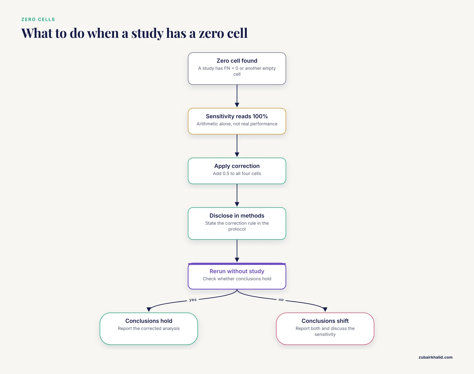
Decide the zero-cell policy before running. Write the correction rule into your protocol so it applies uniformly.
Run a univariate model alongside the bivariate one. If the two disagree sharply, hunt for data problems before hunting for biology.
Keep different reference standards separate. The FilmArray analysis ran distinct models for a culture-based reference standard and for adjudicated final diagnosis, because pooling across them would blur the question [1].
Use meta-regression sparingly. With few studies, each covariate costs power. Prespecify a small set of candidate moderators rather than testing everything.
Save the script or session. A saved R script or exported Meta-DiSc session makes the analysis reproducible when reviewers ask for changes.

Common Mistakes and Limitations

Flowchart for a study with a zero cell: add 0.5 to all four cells, disclose it, then rerun without the corrected study to check conclusions.

Swapping the FP and FN columns. The pooled estimates then look implausibly good and the summary point can fall outside the cloud of study points. Fix: recompute two studies by hand as in Step 2 before running the model.
Pooling sensitivity and specificity as independent proportions. Older workflows applied DerSimonian-Laird pooling to each measure separately and drew a Moses-Littenberg SROC line, and a recent methods guide shows this traditional route can yield biased, clinically misleading estimates compared with hierarchical models [2]. Fix: use a bivariate or HSROC model in any current tool.
Ignoring threshold differences. Sensitivities compared across studies at different cutoffs do not measure the same quantity. Fix: record cutoffs, interpret accuracy through the SROC framework, and consider subgroups by threshold only when studies are numerous.
Handling zero cells silently. A study with FN = 0 shows a sensitivity of 100 percent by arithmetic alone. Fix: apply the standard 0.5 continuity correction to all four cells of that table, disclose it in your methods, and rerun the analysis without the corrected study to confirm your conclusions hold.
Reading the confidence ellipse as a prediction ellipse. The confidence region describes uncertainty in the summary point, while the prediction region describes where a new study would land [4]. Fix: report both and label them explicitly.
Treating AUC as clinical usefulness. AUC ignores prevalence and the asymmetric costs of false positives and false negatives. Predictive values shift with prevalence even when sensitivity and specificity hold steady [14]. Fix: report likelihood ratios and discuss pretest probability in your interpretation.
Skipping risk-of-bias appraisal. Accuracy studies are prone to design flaws such as partial verification and inappropriate exclusion of indeterminate results, which is why QUADAS-2 exists. Fix: complete QUADAS-2 for every study before pooling.
Meta-regression fishing with too few studies. Each added covariate consumes degrees of freedom, and unstable covariate estimates produce spurious explanations for heterogeneity. Fix: prespecify a small number of moderators and treat exploratory findings as hypothesis-generating.

A pooled estimate describes average performance across the included studies. It does not tell you what the test will do in your laboratory, with your prevalence, or with your operators, and individual diagnostic decisions always require clinical judgment alongside the numbers.

Frequently Asked Questions

What is a diagnostic test accuracy meta-analysis calculator?

It is a tool that pools sensitivity and specificity from multiple primary studies using a bivariate random-effects model. It outputs pooled estimates with confidence intervals, an SROC curve, and heterogeneity statistics such as the bivariate I-squared and prediction ellipse.

What data do I need before I start?

You need the four cell counts from each primary study's 2 x 2 table: true positives, false positives, false negatives, and true negatives. Each study must compare the same index test against a defined reference standard.

Which calculator should I use?

Meta-DiSc 2.0 works well for point-and-click analysis in a browser, MetaDTA is another free option, and R with the mada package gives you scripted, reproducible runs. Stata users can use the metandi, midas, or metadta commands. All of them implement bivariate or hierarchical models.

Why can I not just average sensitivity and specificity across studies?

Simple averages ignore the fact that sensitivity and specificity trade off against each other when studies use different thresholds. The bivariate model estimates both outcomes and their correlation at the same time, which gives more honest pooled estimates and intervals.

How many studies do I need?

There is no fixed cutoff, but the bivariate model must estimate between-study variances, so very small sets give unstable results. A methodological review found that formal heterogeneity investigations become more common as the number of primary studies grows.

What does the SROC curve tell me?

It summarizes the tradeoff between sensitivity and false positive rate across studies. The area under the curve gives a single measure of discrimination, where 1.0 is perfect separation of diseased and disease-free patients.

How do I handle a study with a zero cell?

Add 0.5 to all four cells of that study's table, the standard continuity correction, and disclose it in your methods. Then rerun the analysis without the corrected study to confirm your conclusions hold.

How should I report the results?

Follow the PRISMA-DTA checklist and report pooled sensitivity and specificity with 95% confidence intervals, the SROC area, heterogeneity statistics, QUADAS-2 risk-of-bias judgments, and a publication bias assessment such as Deek's funnel plot test.