How to Convert Month to Number in Excel (Step by Step)

By Dr. Zubair Khalid, DVM, MS, PhD · 2026-10-03

Converting a month to number in Excel means turning a text label like "January" into its numeric position, 1. The most reliable way is to combine the month name with a day, convert that text into a real date, then read the month with the MONTH function. This article shows the exact formula, a worked example, and the alternatives when your data does not behave.

Quick Answer

The core formula is =MONTH(DATEVALUE(A2&" 1")), which returns 1 for "January" and 12 for "December".
DATEVALUE cannot read a bare month name, so you append a day to the month name before converting. Excel fills in the current year.
MONTH then extracts the month position from that date serial number.
A lookup table with =MATCH(A2,{"January","February",...},0) works when you want to control the mapping yourself.
If the cell already holds a real date, skip DATEVALUE and use =MONTH(A2) directly.

Before You Start

You need to know what is actually inside the cell. Excel treats "January" typed as text differently from a date formatted to display "January". The two look identical on screen but behave differently in formulas.

To check, click the cell and look at the formula bar. If the formula bar shows something like 1/15/2024 while the cell shows "January", the cell holds a real date and you can use MONTH on it directly. If the formula bar shows the word January, the cell holds text and you need DATEVALUE or a lookup.

You also need to know your regional date settings. DATEVALUE interprets text according to your system's date format, which affects how it reads the string you build. The formula in this article appends a space and the number 1, producing text like "January 1", which Excel reads as the first day of January in the current year.

One more thing worth checking: trailing spaces. A cell containing "January " with a space at the end looks fine but breaks DATEVALUE. The TRIM function removes those characters.

Step by Step

Put your month names in a column. In the example below they sit in column A starting at A2.

In the adjacent cell, build a date text string. Concatenate the month name with a space and the day number 1:

$$=A2 \& " 1"$$

This produces "January 1". DATEVALUE can read that as a date.

Wrap it in DATEVALUE to get a date serial number:

$$=DATEVALUE(A2 \& " 1")$$

Excel returns a number like 45292, which is the internal representation of January 1.

Wrap the whole thing in MONTH to pull out the month position:

$$=MONTH(DATEVALUE(A2 \& " 1"))$$

For "January" this returns 1.

Copy the formula down the column. Relative references adjust automatically, so A3, A4 and so on feed the same logic.

If you are new to building nested formulas, the structure here is a good practice case. The guide to making a formula in Excel walks through how functions nest inside one another.

Worked Example

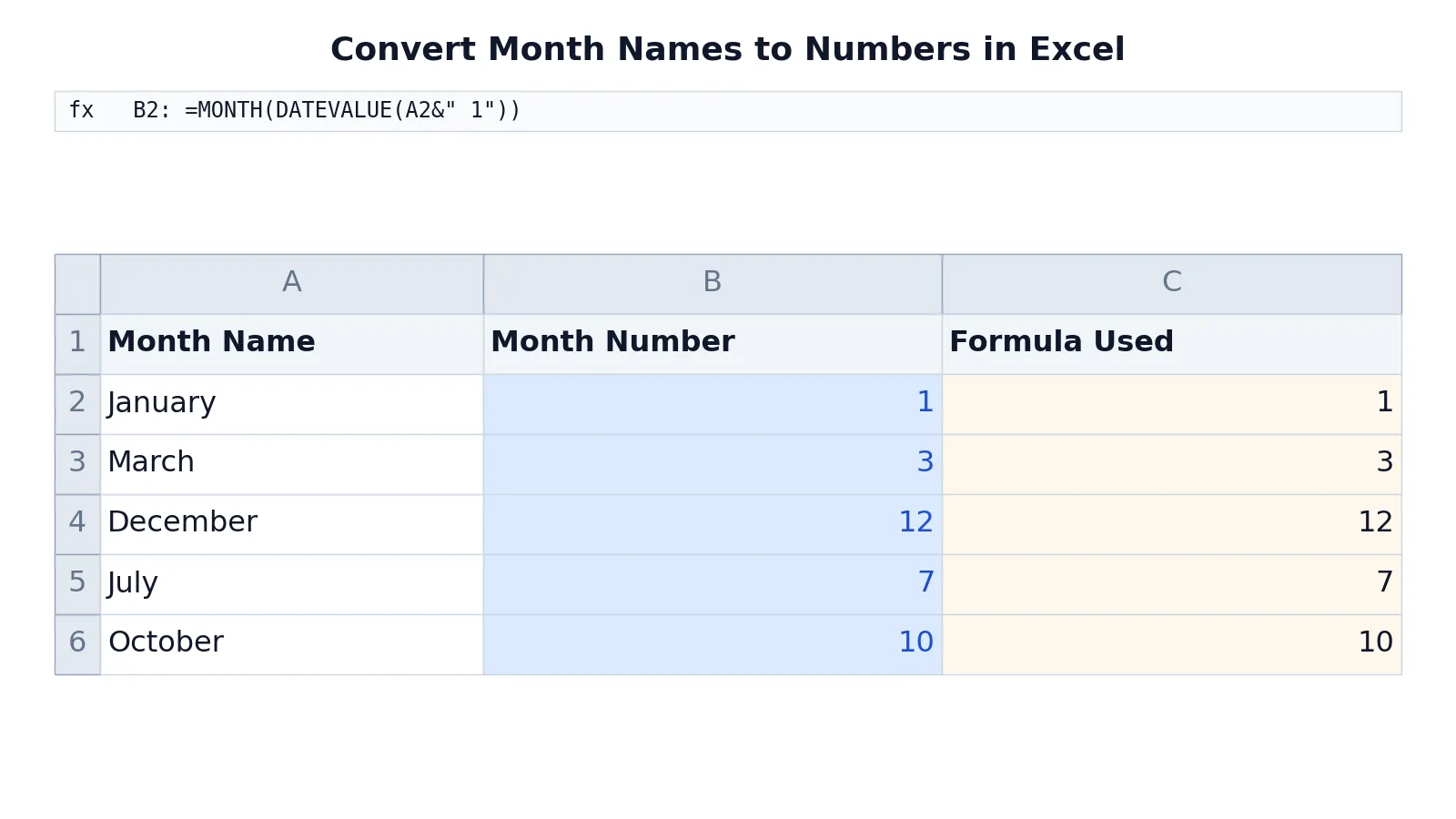
The table below converts five month names to their numbers. Column A holds the text, column B holds the formula and its result, and column C repeats the formula for reference.

	A	B	C
1	Month Name	Month Number	Formula Used
2	January	`=MONTH(DATEVALUE(A2&" 1"))` -> displays 1	`=MONTH(DATEVALUE(A2&" 1"))` -> displays 1
3	March	`=MONTH(DATEVALUE(A3&" 1"))` -> displays 3	`=MONTH(DATEVALUE(A3&" 1"))` -> displays 3
4	December	`=MONTH(DATEVALUE(A4&" 1"))` -> displays 12	`=MONTH(DATEVALUE(A4&" 1"))` -> displays 12
5	July	`=MONTH(DATEVALUE(A5&" 1"))` -> displays 7	`=MONTH(DATEVALUE(A5&" 1"))` -> displays 7
6	October	`=MONTH(DATEVALUE(A6&" 1"))` -> displays 10	`=MONTH(DATEVALUE(A6&" 1"))` -> displays 10

The formula does two jobs in sequence. First it combines the month name with a space and 1 to create a date text, then converts that text to a date serial number. Second it extracts the month number from that serial number. The same formula copied down handles March, December, July and October without any edits.

Notice that the day value you append does not change the result. Any valid day works because you only read the month back out. Using 1 keeps the string short and avoids month-end edge cases.

Other Ways to Do It

The MONTH and DATEVALUE combination is not the only route. Pick based on your data and how much control you want.

Lookup with MATCH. If you want an explicit mapping, list the twelve month names in order and use MATCH to find the position:

$$=MATCH(A2,\{"January","February","March","April","May","June","July","August","September","October","November","December"\},0)$$

The 0 argument forces an exact match. This returns 1 for January and 12 for December. It is transparent and easy to audit, and it does not depend on regional date settings.

Lookup with a reference table. Put the twelve names in one range and the numbers 1 to 12 beside them, then use VLOOKUP or XLOOKUP against that range. This is the better choice when the month names come from a source you do not control and might include abbreviations.

MONTH on a real date. If the cell already contains a date, the formula is simply =MONTH(A2). No DATEVALUE needed. This is the cleanest case and the one you should aim for when importing data.

TEXT and VALUE for numeric month strings. If your cell contains "01" or "1" as text, =VALUE(A2) converts it to a number. This is a different problem from month names, and the text to number conversion guide covers the general techniques.

Abbreviations. DATEVALUE reads "Jan 1" as January 1 in most configurations, so the same formula often works for three-letter month names. Test it on your own data before relying on it, because abbreviated forms are more sensitive to regional settings than full names.

Once you have month numbers, they feed naturally into other date calculations. If you need to count how many days a given month has, the days in a month guide shows the formula. If you are measuring the gap between two dates in months, see months between two dates.

Troubleshooting

The formula returns #VALUE! DATEVALUE could not read the text as a date. Check for trailing spaces, a misspelled month name, or a cell that contains something other than a month. Wrap the reference in TRIM: =MONTH(DATEVALUE(TRIM(A2)&" 1")).

The formula returns the wrong month. This usually means the cell holds a real date that you did not expect, or the text includes extra words. Look at the formula bar to confirm what is stored.

The formula returns a date instead of a number. The cell is formatted as a date. Change the number format to General or Number. The underlying value is already correct.

The formula works for some rows and fails for others. Mixed data. Some cells hold text, some hold dates. Sort or filter to find the outliers, then normalize the column.

Results change when you open the file on another computer. Regional date settings differ between machines. The lookup approach avoids this entirely because it does not parse dates.

Common Mistakes

Forgetting the day. =MONTH(DATEVALUE(A2)) fails because DATEVALUE cannot read a bare month name. Append a space and 1.
Using MONTH on a text cell. =MONTH(A2) returns #VALUE! when A2 contains the word January. MONTH expects a date serial number, not text.
Leaving trailing spaces in the source data. "January " breaks DATEVALUE. Clean the column with TRIM before converting.
Assuming the result is text. The formula returns a real number. If it looks like a date, the cell format is wrong, not the formula.
Hardcoding month names in a lookup without checking case. MATCH is not case sensitive, so "january" and "JANUARY" both match "January", but a misspelling does not. Verify your source values.
Copying the formula without checking references. If you used absolute references by accident, every row returns the same month. Confirm the row reference changes as you copy down.

Limitations

The DATEVALUE approach depends on your system's regional date settings. A formula that works on your machine can return #VALUE! or a different month on a colleague's machine if the locale interprets date text differently. For shared workbooks, a lookup table is safer because it does not parse dates at all.

The method also assumes clean, consistent input. It handles full month names and, in most configurations, standard three-letter abbreviations. It does not handle misspellings, mixed languages, ordinal forms like "1st month", or cells that combine a month with other text. When your source data is messy, fix the data first. A formula layered on top of inconsistent text produces inconsistent results.

Frequently Asked Questions

Why does MONTH alone not work on a month name?

MONTH expects a date serial number, which is how Excel stores dates internally. A text string like "January" is not a serial number, so MONTH returns #VALUE!. You need to convert the text to a date first, which is what DATEVALUE does.

Does the day I append matter?

No. You only read the month back out, so any valid day produces the same result. Using 1 keeps the string short and avoids edge cases at the end of short months.

Can I convert abbreviated month names like Jan?

In most configurations, yes. DATEVALUE reads "Jan 1" as January 1, so =MONTH(DATEVALUE(A2&" 1")) returns 1. Abbreviations are more sensitive to regional settings than full names, so test on your own machine before rolling the formula out.

What if my cell already contains a date?

Use =MONTH(A2) directly. The cell already holds a serial number, so no conversion is needed. Check the formula bar to confirm the cell holds a date and not text.

How do I convert the number back to a month name?

Use the TEXT function with a month code: =TEXT(DATE(2024,A2,1),"mmmm") returns the full name, and "mmm" returns the abbreviation. The DATE function builds a valid date from the month number you supply.

References

This article draws on the standard references listed under Further Reading.