LC-MS and LC-MS/MS: How They Work
By Dr. Zubair Khalid, DVM, MS, PhD ·
Liquid chromatography mass spectrometry is a two-stage measurement. The liquid chromatography half separates molecules in time. The mass spectrometry half separates ions by mass-to-charge ratio and counts them. Put the two together and you can identify and quantify a specific compound inside a complex biological matrix, often at concentrations in the low nanograms per milliliter.
By the end of this guide you will be able to trace a sample through every physical step of an LC-MS or LC-MS/MS run, explain the difference between single-stage and tandem instruments, define multiple reaction monitoring in plain language, and read an LC-MS chromatogram the way a clinical laboratory scientist reads one. You will also know which failures produce which artifacts, so a bad peak tells you where to look.
What you need on hand to follow the worked examples: a basic understanding of how a reversed-phase column retains analytes, comfort with the idea of a mass-to-charge ratio, and a willingness to think in units. Retention time is reported in minutes. Mass-to-charge ratio is reported as m/z, which is dimensionless in practice. Analyte concentration is reported in ng/mL or µg/mL. Those three numbers, plus peak area, are the language of this technique.
The Big Picture: Separation Then Measurement
An LC-MS instrument is a pipeline. A liquid sample enters an autosampler. A pump pushes it through a column packed with chemically modified particles. Compounds leave the column at different times because they partition differently between a liquid mobile phase and a solid stationary phase. Each compound then enters an ionization source, where it becomes a gas-phase ion. Those ions travel into a mass analyzer that filters or sorts them. A detector counts the ions that survive the trip. Software turns the counts into a chromatogram, which is a plot of signal intensity against time.
The reason the two stages exist is that neither one alone is enough. Liquid chromatography alone gives you retention time, which is a weak identifier in a complex matrix. Many compounds can co-elute at the same time. Mass spectrometry alone gives you a mass spectrum, but if you inject a whole blood extract directly, thousands of compounds compete for charge and the signal is a mess. Coupling them means the mass spectrometer only sees what the column delivers at a given moment, and the column only has to resolve the compounds that matter from their nearest neighbors.
This is why the technique dominates therapeutic drug monitoring, toxicology, biomarker research, and reference measurement procedures. An isotope dilution LC-MS/MS method for gentamicin in human serum can be validated against quantitative nuclear magnetic resonance to establish traceability to the International System of Units, with within-run precision reported as a coefficient of variation of 0.2 to 0.9 percent [1]. That level of control is not achievable with a single separation dimension.
Step 1: Sample Preparation and Injection
Before the column sees anything, the matrix has to be tamed. Whole blood, serum, plasma, urine, and tissue homogenates contain proteins, salts, phospholipids, and pigments that will foul the column and suppress ionization. The standard approaches are protein precipitation, solid-phase extraction, and online extraction.
A representative whole-blood toxicology method precipitates proteins with a 1:1 mixture of acetonitrile and methanol, centrifuges, filters, and injects 1 µL onto a C18 column at a flow rate of 0.4 mL/min [2]. A semaglutide assay in rat plasma uses acetone-mediated protein precipitation followed by solid-phase extraction, injecting 50 µL of plasma and separating on a C18 column within 9 minutes [3]. Online approaches couple a trap column or a monolithic oligosorbent directly to the analytical column, which reduces manual steps and improves reproducibility. An online aptamer-based solid-phase extraction coupled to HPLC-MS achieved lower limits of quantification down to 0.03 ng/mL for amyloid-β peptides in cerebrospinal fluid, with coefficients of variation from 1.1 to 6.2 percent for Aβ40 [4].
The practical point is that sample preparation determines your lower limit of quantification more often than the mass spectrometer does. Cleaner extracts mean less ion suppression and lower background.
Step 2: Liquid Chromatography Separation
The column is the heart of the separation. Most clinical and bioanalytical methods use reversed-phase chromatography on a C18 stationary phase, meaning the stationary phase is nonpolar and the mobile phase is polar. Analytes partition into the nonpolar stationary phase to varying degrees. More hydrophobic compounds retain longer. More polar compounds elute earlier.
Mobile phases are usually water and an organic solvent such as acetonitrile or methanol, each modified with a volatile acid or buffer. Formic acid at 0.1 percent is common because it supplies protons for positive-mode ionization and keeps the pH low enough to suppress silanol interactions. Ammonium acetate at 5 mmol/L is used when a volatile buffer is needed. A representative alkaloid method uses 0.1 percent formic acid in acetonitrile, 0.1 percent formic acid in water, and 5 mmol/L ammonium acetate in a gradient [2].
Gradient elution is standard. The instrument starts at a low organic percentage and ramps it up over the run. Early-eluting polar compounds separate while the organic strength is low. Later, the increasing organic content pushes hydrophobic compounds off the column in a sharp band. Gradient elution compresses peak widths for late-eluting analytes and shortens total run time.
Retention time is the clock reading at which an analyte exits the column, reported in minutes. It is the first line of identification. A compound that should appear at 4.2 minutes but appears at 4.2 minutes in the calibrator and 4.9 minutes in the patient sample is not the same signal, or the chromatography has shifted. Retention time is not a physical constant. It depends on column age, mobile phase composition, temperature, and flow rate. This is why every batch runs calibrators and quality control samples interspersed with unknowns.
Step 3: Ionization
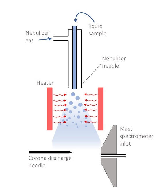

The column effluent is a liquid at atmospheric pressure. The mass analyzer operates under high vacuum and needs gas-phase ions. The interface between them is the ionization source. Electrospray ionization is the dominant technique for polar and semipolar compounds.
In electrospray ionization, the liquid passes through a narrow capillary held at a high potential, typically a few kilovolts. The electric field pulls the liquid into a fine spray of charged droplets. A heated drying gas evaporates solvent from each droplet. As the droplet shrinks, the charge density rises until Coulomb repulsion ejects ions into the gas phase. Those ions are then sampled into the vacuum region of the mass spectrometer.
Electrospray ionization is soft. It adds or removes a proton rather than shattering the molecule. A neutral analyte M in positive mode becomes a protonated molecule at m/z equal to the neutral mass plus 1.008, written [M+H]+. In negative mode it becomes [M-H]-, the neutral mass minus 1.008. Larger molecules such as peptides pick up multiple protons and appear as a series of multiply charged ions. Semaglutide, a peptide, is monitored as m/z 1029.4 in positive mode [3]. Multiply charged ions are the norm for peptides and proteins and are useful because they extend the effective mass range of the analyzer.
Ionization is not perfectly reproducible across instruments and laboratories. A multi-laboratory study of an internal retention time standard mixture across ten laboratories and four instrument vendors found variation in the ion species formed, even when extraction and chromatography protocols were standardized [5]. The lesson for the bench is that source conditions, solvent composition, and ion optics shape which ions you actually see. Method transfer between sites requires re-optimization, not just copying parameters.
Step 4: Mass Analysis
Once ions are in the gas phase, the mass analyzer sorts them by mass-to-charge ratio. Several analyzer designs are in routine use, and each has a different job.
A quadrupole is a set of four parallel metal rods. Applying a combination of radiofrequency and direct-current voltages to the rods creates a filter that transmits only ions in a narrow m/z window. Change the voltages and you change the window. A quadrupole is fast, robust, and inexpensive to operate, but it has low mass resolution. It cannot distinguish two ions that differ by a small fraction of a dalton.
A triple quadrupole places three quadrupoles in series. The first quadrupole selects a precursor ion. The second quadrupole is a collision cell filled with an inert gas such as nitrogen or argon, where the precursor is fragmented by collision-induced dissociation. The third quadrupole selects a product ion. This arrangement is the workhorse of quantitative bioanalysis.
A time-of-flight analyzer accelerates ions into a flight tube and measures how long they take to reach the detector. Lighter ions arrive first. Time-of-flight instruments give high resolution and accurate mass, which supports molecular formula assignment.
An Orbitrap traps ions in an electrostatic field and measures their oscillation frequencies. Fourier transformation of the detected signal produces a high-resolution mass spectrum. An HPLC-ESI-Orbitrap method measured the carbon isotopic composition of perfluorooctanoic acid with offsets from reference values between 0.2 and 1.1 parts per thousand and errors between 0.8 and 1.5 parts per thousand [6]. That is high-resolution work at the isotopic level.
The choice of analyzer follows the question. Quantify one known compound at low concentration in a messy matrix and you want a triple quadrupole in MRM mode. Identify an unknown metabolite or confirm a molecular formula and you want high-resolution accurate mass.
Step 5: Detection and Signal Generation
The detector converts arriving ions into electrical current. An electron multiplier or a conversion dynode plus multiplier produces a cascade of electrons for each ion impact. The result is a count, and the count over time is the signal.
Software plots signal intensity on the vertical axis against retention time in minutes on the horizontal axis. That plot is the LC-MS chromatogram. Each analyte appears as a peak. The area under that peak is proportional to the number of ions detected, which is proportional to the amount of analyte that entered the source, which is proportional to the concentration in the injected sample, provided the calibration holds.
In MRM mode, the instrument does not scan. It sits on a single precursor-to-product transition and records the ion current for that transition continuously. That is why MRM chromatograms are clean. The instrument is blind to everything that does not fragment from the selected precursor into the selected product.
Single-Stage LC-MS Versus Tandem LC-MS/MS
Single-stage LC-MS uses one mass analyzer. The analyzer might scan across a range of m/z values to produce a full mass spectrum at each point in the chromatogram, or it might sit on a single m/z value to monitor one ion. Single-stage instruments are useful for confirmation, for screening when the analyte list is open-ended, and for high-resolution accurate-mass work where the exact mass itself is the identifier.
Tandem LC-MS/MS uses two stages of mass analysis with fragmentation in between. The first analyzer selects a precursor. The collision cell fragments it. The second analyzer selects a product. This is the defining feature of the technique.
The power of tandem mass spectrometry is selectivity. A single-stage instrument distinguishes compounds by retention time and m/z. A tandem instrument distinguishes them by retention time, precursor m/z, and product m/z. Two compounds that share a precursor mass but fragment differently are resolved. Two compounds that fragment identically but differ in precursor mass are resolved. The combination of three orthogonal properties makes false positives rare.
Tandem mass spectrometry also improves signal-to-noise. Chemical background that happens to sit at the precursor m/z usually does not fragment into the product m/z you are monitoring. The background is filtered out twice.
MRM: Precursor to Product Ion Monitoring
Multiple reaction monitoring, abbreviated MRM, is the acquisition mode that defines quantitative LC-MS/MS. The name describes exactly what happens. The instrument monitors one or more specific reactions, where a reaction is the conversion of a precursor ion into a product ion inside the collision cell.
The notation is written as precursor m/z → product m/z. The semaglutide assay monitors m/z 1029.4 → 110.1 for the analyte and m/z 938.9 → 109.9 for liraglutide, the internal standard [3]. A method for 37 alkaloids in whole blood uses MRM in positive electrospray mode with a matrix-matched external calibration curve, achieving detection limits from 0.01 to 2.50 ng/mL and quantification limits from 0.03 to 7.50 ng/mL [2]. A piperacillin reference measurement procedure operates in positive electrospray ionization and MRM mode across a range of 0.400 µg/mL to 240 µg/mL [7].
Two concepts matter for reading MRM data.
The quantifier transition is the one used to calculate concentration. It is chosen for sensitivity and freedom from interference. The qualifier transition is a second product ion from the same precursor. The ratio of quantifier to qualifier peak area is a confirmation criterion. If the ratio in a patient sample differs from the ratio in the calibrator, an interfering compound is probably contributing to the signal.
Dwell time is how long the instrument spends on each transition before moving to the next. More transitions per method means less dwell time per transition, which reduces the number of data points across a peak. Too few points and the peak shape is distorted and integration becomes unreliable. This is the practical ceiling on how many analytes you can multiplex in one run. A 37-alkaloid panel is a large multiplex, and the method compensates with a fast gradient and a short column.
The following diagram traces the decision path from injection to a reported result.
flowchart TD
    A[Sample injection] --> B[LC column separation]
    B --> C[Electrospray ionization]
    C --> D{Analyzer mode}
    D --> E[Single stage scan]
    D --> F[Precursor selection]
    F --> G[Collision cell fragmentation]
    G --> H[Product selection MRM]
    E --> I[Detector]
    H --> I
    I --> J[Chromatogram peak]
    J --> K{Peak acceptable}
    K --> L[Integrate and quantify]
    K --> M[Investigate interference]
Reading an LC-MS Chromatogram
A chromatogram is a graph, and reading it is a skill. Work through the following properties in order every time.
Retention Time
Locate the peak apex on the time axis. Record it in minutes to two decimal places. Compare it to the retention time of the calibrator and the internal standard in the same batch. The internal standard is the anchor. If the internal standard retention time has shifted, the chromatography has drifted and every analyte retention time will shift with it. If the internal standard is stable but the analyte has moved, suspect an interference or a matrix problem specific to that sample.
Peak Area
Peak area is the integrated signal across the peak, measured from baseline to baseline. Area is preferred over peak height for quantification because it is less sensitive to band broadening and small shifts in retention time. The ratio of analyte area to internal standard area is the response used in the calibration curve. Isotope-labeled internal standards are the gold standard because they co-elute with the analyte and experience the same ionization conditions. A structural analog internal standard, such as C2-D3 used to quantify gentamicin isomers, is a reasonable alternative when a labeled version is unavailable [1].
Signal-to-Noise
Signal-to-noise ratio compares the analyte peak height to the short-term noise of the baseline in a blank region adjacent to the peak. It is the conventional way to express detection capability. A method reporting detection limits from 0.01 to 2.50 ng/mL is reporting the concentrations at which the signal-to-noise ratio reaches the laboratory's chosen threshold [2]. Signal-to-noise is not a property of the analyte alone. It depends on the noise, and noise depends on the cleanliness of the extract and the age of the source.
Baseline and Integration
The baseline is the signal level where no analyte is eluting. Draw it under the peak from a flat region before the peak to a flat region after it. Integration software does this automatically, but automatic integration fails in predictable ways. A sloping baseline from a late-eluting matrix component will inflate the area. A baseline drawn through a small interfering peak will deflate it. Inspect every integration manually, especially near the lower limit of quantification.
Co-elution
Co-elution means two compounds leave the column at the same time. In single-stage LC-MS, co-elution is a serious problem because the mass analyzer may not resolve them. In MRM mode, co-elution is tolerable if the interfering compound does not share both the precursor and the product transition. This is the practical reason tandem mass spectrometry is preferred for complex matrices. The qualifier-to-quantifier ratio is your check. A ratio outside the expected range is evidence of co-elution with an isobaric interferent.
Peak Shape
A good peak is roughly Gaussian, with a rise, an apex, and a symmetric fall. Fronting (a leading edge that rises too slowly) suggests column overload or a solvent mismatch between the injection solvent and the mobile phase. Tailing (a trailing edge that falls too slowly) suggests secondary interactions with residual silanols or a dead volume problem in the plumbing. Splitting suggests a partially blocked frit or a bad connection.
The Table: Component, Function, Failure Mode
| Component | Function | Failure mode and what you see |
|---|---|---|
| Autosampler | Draws and injects a defined volume | Carryover from a previous high-concentration sample, seen as a small peak at the analyte retention time in the blank |
| LC pump | Delivers mobile phase at a controlled flow and gradient | Gradient drift or pulsation, seen as retention time shifts and baseline ripple |
| Analytical column | Separates analytes by partition | Column aging, seen as loss of resolution, peak tailing, and rising backpressure |
| Ionization source | Converts liquid-phase analyte to gas-phase ions | Source fouling, seen as falling response across the batch and rising variability |
| First quadrupole | Selects the precursor ion | Incorrect or drifting mass calibration, seen as loss of signal on the correct transition |
| Collision cell | Fragments the precursor by collision-induced dissociation | Contamination or gas pressure drift, seen as altered product ion ratios |
| Second quadrupole | Selects the product ion | Same as first quadrupole, plus cross-talk between transitions |
| Detector | Converts ions to electrical current | Detector fatigue, seen as nonlinear response at high concentrations |
| Data system | Integrates peaks and calculates concentration | Misintegration, seen as area errors that do not match visual inspection |
Worked Example: From Raw Data to a Reported Concentration
Suppose you are quantifying a drug in serum by LC-MS/MS with an isotope-labeled internal standard. You have a six-point calibration curve, a blank, a zero standard, and quality control samples at three levels. Your instrument reports peak areas.
Step 1. Confirm retention time. The analyte should appear at 3.45 minutes and the internal standard at 3.42 minutes. Both are within 0.05 minutes of the calibrator values. Accept.
Step 2. Check the qualifier ratio. The quantifier-to-qualifier area ratio in the calibrators averages 4.2 with a range of 4.0 to 4.4. Your patient sample gives 4.1. Accept.
Step 3. Calculate the response ratio.
Analyte peak area        = 18,450
Internal standard area   = 52,300
Response ratio           = 18,450 / 52,300 = 0.3528
Step 4. Apply the calibration curve. The curve was fit by weighted linear regression with the equation y = 0.0071x + 0.0012, where y is the response ratio and x is concentration in ng/mL.
0.3528 = 0.0071x + 0.0012
0.3516 = 0.0071x
x = 49.5 ng/mL
Step 5. Check against the quality controls. The low control at 10 ng/mL reported 9.6 ng/mL (96 percent of target). The mid control at 50 ng/mL reported 50.8 ng/mL (102 percent). The high control at 400 ng/mL reported 388 ng/mL (97 percent). All within the laboratory's acceptance window. The batch is valid.
Step 6. Report 49.5 ng/mL, or round to 50 ng/mL depending on the laboratory's significant figures policy.
That sequence, retention time, ratio, area, calibration, quality control, is the same every time. It does not change with the analyte.
Common Mistakes and Limitations
Matrix effects are the most common source of silent error. The matrix is everything in the sample that is not the analyte. Co-eluting matrix components can change the efficiency of droplet formation and ion release in the electrospray source. The result is ion suppression, a reduction in signal, or less commonly ion enhancement. Matrix effects are evaluated by comparing the response of a spiked post-extraction sample to a neat standard. A well-behaved method shows matrix effects close to 100 percent. A semaglutide assay reported matrix effects from 96.34 to 104.12 percent across quality control levels [3]. A piperacillin reference procedure demonstrated matrix independence across serum and plasma [7]. When matrix effects are large and variable, isotope-labeled internal standards compensate because they experience the same suppression as the analyte.
Ion suppression is matrix effect in the direction of lost signal. It is worse when the analyte elutes in a region where many matrix components elute, which is often early in the gradient for polar compounds and in the phospholipid region for plasma extracts. Moving the analyte retention time away from the suppression zone by adjusting the gradient is a standard fix.
Isobaric interference is the presence of a compound with the same nominal mass as the analyte. Isobaric compounds differ in exact mass by small amounts, so high-resolution instruments can separate them while low-resolution quadrupoles cannot. In MRM mode, an isobaric interferent that fragments into the same product ion will be indistinguishable from the analyte. This is why two transitions are monitored and the ratio is checked. It is also why chromatographic separation still matters even on a tandem instrument.
Carryover is analyte left in the autosampler or the injector from a previous sample. It shows up as a peak in the blank or in a low-concentration sample that follows a high one. Carryover is a particular risk when the analytical range spans several orders of magnitude. A semaglutide method spanning 1 to 500 ng/mL reported no carryover [3]. A method for areca nut alkaloids explicitly evaluated carryover as part of validation [8]. The practical fix is a wash step between injections, a stronger wash solvent, or a smaller injection volume.
Calibration drift is a slow change in response over the course of a batch. It can come from source fouling, detector fatigue, or a change in mobile phase composition as the solvent bottles empty. Drift is detected by bracketing the batch with calibrators and running quality controls throughout. If the closing calibrator response differs from the opening calibrator response by more than the laboratory's acceptance window, the batch is suspect. Electric field modulation of the electrospray plume has been explored as a way to correct for instrumental drift during extended analyses [9].
Co-elution of an internal standard with an interfering compound is a subtle problem. The internal standard is supposed to correct for extraction recovery and ionization variability. If something co-elutes with it and adds to its signal, the correction is wrong. This is why internal standards are chosen to elute in a clean region of the chromatogram.
Column contamination accumulates over hundreds of injections. The first sign is usually increased backpressure, followed by peak tailing and loss of resolution for late-eluting analytes. A guard column extends analytical column life. A defined column wash and re-equilibration step at the end of each run reduces the rate of contamination.
The limitations of the technique are worth stating plainly. LC-MS and LC-MS/MS quantify what you tell them to quantify. They do not discover unknown compounds unless you are running a scanning or high-resolution acquisition. A targeted MRM method will report a clean result for a sample that contains a toxic compound outside the panel. Retention time and transition ratio confirm identity only against the compounds you included. Ionization efficiency varies between compounds, so a compound that ionizes poorly will have a higher detection limit than one that ionizes well, even at the same concentration. And every result depends on the calibration curve, the internal standard, and the quality controls being correct. Individual patient results always require interpretation by a qualified laboratory professional and the ordering clinician.
Frequently Asked Questions
What is the difference between LC-MS and LC-MS/MS?
LC-MS uses one stage of mass analysis. LC-MS/MS uses two stages with fragmentation in between, which adds a second mass filter and greatly improves selectivity.
What does MRM stand for?
Multiple reaction monitoring. The instrument monitors specific precursor-to-product ion transitions, one pair of m/z values per transition.
Why is retention time reported in minutes?
Chromatographic runs typically last from about one minute to twenty minutes, so minutes with two decimal places give the resolution needed to compare peaks.
What is m/z?
Mass-to-charge ratio. It is the mass of the ion divided by the number of charges it carries, and it is the quantity a mass analyzer sorts ions by.
What causes ion suppression?
Co-eluting matrix components that interfere with droplet formation or ion release in the electrospray source, reducing the number of analyte ions that reach the detector.
Why do methods use isotope-labeled internal standards?
They co-elute with the analyte and experience the same extraction losses and ionization conditions, so they correct for both.
How do I know if a peak is real?
Check retention time against the calibrator, check the qualifier-to-quantifier ratio, and confirm the peak is absent or negligible in the blank.
Can LC-MS/MS detect compounds not on the panel?
No. A targeted MRM method only reports the transitions it was programmed to monitor. Unknown compounds require a different acquisition mode.
Related Articles
- Mass Spectrometry Work for Proteins: A Beginner's Guide
- Mass Analyzers in Protein Mass Spectrometry
- Mass Spectrometry to Identify Proteins: A Practical Guide
- Protein Quantification Mass Spectrometry: A Practical Guide
- Troubleshooting Mass Spectrometry Protein Identification
- Cognitive Enhancers: What They Are and How They Work
- Minipreps: How They Work and When to Use Them
- Function of Nerves: How the Nervous System Works
- Indirect Fluorescent Antibody Test: How It Works
Sources
- An isotope dilution-liquid chromatography-tandem mass spectrometry-based candidate reference measurement procedure for the quantification of gentamicin in human serum.
- [[Simultaneous rapid determination of 37 alkaloids in whole blood by high performance liquid chromatography-mass spectrometry/mass spectrometry].](https://pubmed.ncbi.nlm.nih.gov/42533658/)
- Development and Validation of a Liquid Chromatography/Tandem Mass Spectrometry Method for the Quantification of the GLP-1 Analog Semaglutide in Rat Plasma, and Its Application in a Pharmacokinetic Study.
- Online aptamer-based solid-phase extraction coupled with high-performance liquid chromatography-mass spectrometry for the determination of Alzheimer's disease biomarkers.
- Multi-Laboratory Assessment Reveals Variable Ion Species Profiles in Electrospray Ionization Mass Spectrometry.
- Stable Carbon Isotope Analysis of Perfluorooctanoic Acid (PFOA) by Microflow-High Pressure Liquid Chromatography-Orbitrap Mass Spectrometry.
- An isotope dilution-liquid chromatography-tandem mass spectrometry-based candidate reference measurement procedure for the quantification of piperacillin in human serum and plasma.
- Development and application of a liquid chromatography-tandem mass spectrometry method for the analysis of Areca nut alkaloids in rat plasma for a toxicokinetic study.
- Electric Field-Modulated Electrospray Ionization Mass Spectrometry for Quantity Calibration and Mass Tracking.