How to Choose the Right Statistical Test for Your Bioinformatics Data
By Dr. Zubair Khalid, DVM, MS, PhD ·
The difference between most candidate statistical tests comes down to one sentence: a parametric test compares means and leans on the normal distribution for power, while a nonparametric test compares ranks and makes almost no assumption about shape. The rule of thumb for choosing follows directly. Run the parametric test when your outcome is continuous, your observations are independent or correctly paired, and normality is plausible. Switch to its nonparametric counterpart when any of those three conditions fails.
A statistical hypothesis test quantifies whether the pattern in your data is larger than the noise you would expect from sampling alone. It returns a p-value, the probability of seeing a result at least this extreme if the null hypothesis were true, where the null hypothesis is usually the boring statement that the groups share the same underlying distribution. Bioinformatics makes this decision feel harder than it is because measurements arrive in intimidating forms: sequence alignments, expression matrices, proteomics gels, dose metrics, and clinical labels. Translational bioinformatics routinely integrates medications, diseases, and genomes with clinical and pathological features [1], yet the statistical question underneath is almost always one of three things: a comparison between groups, an association between variables, or a performance check between models.
If you are deciding which statistical test to use for bioinformatics data in Python, the decision is more mechanical than it looks. This guide gives you a three-question workflow, a master selection table, the exact Python entry point for every standard test, worked scenarios modeled on real study designs, and the mistakes that most often invalidate an otherwise correct analysis. The code targets the core stack for Python for bioinformatics work: scipy, statsmodels, scikit-learn, and Biopython.
The Three Questions That Decide Every Test
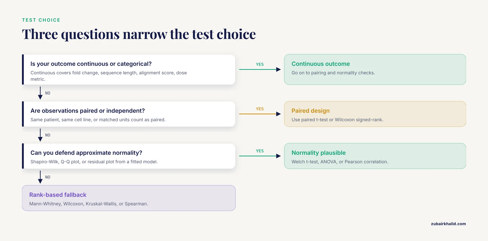
Every test-choice problem reduces to three questions about your data. Answer them in order and the options collapse from dozens to one or two.
Question 1: What Type of Outcome Did You Measure?
The outcome variable, sometimes called the dependent variable, is the measurement your hypothesis is about. In bioinformatics it usually falls into one of these classes:
- Continuous: expression fold change, sequence length, alignment score, deuterium uptake percentage, dose metric. These call for t-tests, ANOVA, correlation, or regression.
- Categorical: mutation present or absent, resistant or susceptible, benign or malignant class label. These call for chi-square, Fisher's exact, McNemar, or Cochran's Q.
- Ordinal or rank-based: stage scores, ordered confidence ratings. Treat these like non-normal continuous data and reach for rank-based tests.
Question 2: Are Your Observations Independent or Paired?
Observations are paired when two measurements come from the same biological unit or from units deliberately matched to each other. The same patient before and after treatment, the same cell line under two conditions, the same treatment plan rebuilt by two planning systems, and matched case-control pairs are all paired designs. Observations are independent when each measurement comes from a different, unrelated unit.
Pairing changes the test because a paired design lets each unit serve as its own control, which strips out between-unit variability. The paired t-test and the Wilcoxon signed-rank test are the paired counterparts of the two-sample t-test and the Mann-Whitney U test. Choosing the unpaired test on paired data throws away most of your statistical power. Choosing the paired test on independent data inflates your false positive rate.
Question 3: Can You Defend the Distribution Assumptions?
Parametric tests assume the data, or more precisely the residuals, follow an approximately normal (Gaussian, bell-shaped) distribution, and several of them also assume similar variances across groups. Check this with a Shapiro-Wilk test on each group, a quantile-quantile plot, or a residual plot from a fitted model.
from scipy import stats

stats.shapiro(group_a)          # p > 0.05 is consistent with, not proof of, normality
stats.levene(group_a, group_b)  # checks similar variances across groups
Two cautions apply. With five or ten observations per group, the Shapiro-Wilk test has almost no power to detect non-normality, so a high p-value there is weak evidence. With hundreds of observations, normality matters far less because the parametric tests behave well anyway. In practice, small bioinformatics validation sets skew toward the nonparametric column, and large omics datasets tolerate the parametric column.
Plan the Sample Size Before You Test
Power is the probability that a test detects a real effect of a given size. Alpha is the false positive rate you accept, conventionally 0.05. The type II error rate (beta) is the miss rate, and power equals 1 minus beta. Published two-group comparisons commonly justify their sample size with a formal power analysis. One published two-model comparison set power at 80 percent, alpha at 0.05, and beta at 0.2, which produced 10 samples per group. You can reproduce that arithmetic in Python:
from statsmodels.stats.power import TTestIndPower

n_per_group = TTestIndPower().solve_power(effect_size=0.8, alpha=0.05, power=0.8)
The effect_size argument is Cohen's d, the standardized difference between two means. By Cohen's conventional thresholds, 0.8 is a large effect, 0.5 medium, and 0.2 small.
Which Statistical Test to Use in Bioinformatics with Python: The Master Table
The table below is the core of this article. Find the row that matches your three answers and you have your test, its Python entry point, and the failure mode to avoid.
| Your question | Data situation | Test | Python entry point | Check before trusting it | Classic failure |
|---|---|---|---|---|---|
| Do two independent groups differ in their means? | Continuous outcome, two groups, roughly normal | Welch's t-test | scipy.stats.ttest_ind(a, b, equal_var=False) | Approximate normality per group, especially at small n | Using Student's t-test with unequal variances and unequal group sizes |
| Do two independent groups differ, with no distribution guarantee? | Continuous or ordinal, skewed, outliers, tiny n | Mann-Whitney U | scipy.stats.mannwhitneyu(a, b) | Similar distribution shapes if you want to speak about medians | Calling it a medians test when the shapes differ |
| Did the same units change between two conditions? | Continuous, paired measurements | Paired t-test | scipy.stats.ttest_rel(before, after) | Normality of the paired differences | Testing the two conditions as separate groups |
| Same question, non-normal differences | Paired, skewed differences | Wilcoxon signed-rank | scipy.stats.wilcoxon(before, after) | Roughly symmetric differences | Not reporting how zero-difference pairs were handled |
| Do three or more group means differ? | Continuous, 3+ independent groups | One-way ANOVA | scipy.stats.f_oneway(g1, g2, g3) | Normal residuals, similar variances | Reporting the omnibus F without post-hoc pairwise tests |
| Same question, non-normal | 3+ groups, skewed or ordinal | Kruskal-Wallis | scipy.stats.kruskal(g1, g2, g3) | Independent observations | Skipping the Dunn post-hoc comparisons |
| Are two categorical labels associated? | Counts in a contingency table | Chi-square test | scipy.stats.chi2_contingency(table) | Expected count of at least 5 in most cells | Applying it to small or sparse counts |
| Same question with small counts | 2x2 table or sparse larger table | Fisher's exact test | scipy.stats.fisher_exact([[a, b], [c, d]]) | None beyond independent sampling | Reaching for chi-square out of habit at small n |
| Do two continuous variables rise together in a straight line? | Continuous pairs, linear pattern | Pearson correlation | scipy.stats.pearsonr(x, y) | Linearity, no influential outliers | Reading correlation as causation |
| Same question, monotonic but curved, or ordinal | Ranks or monotonic pattern | Spearman correlation | scipy.stats.spearmanr(x, y) | Monotonic relationship | Using it to claim a specific functional form |
| Are any of my thousands of features significant? | One test per feature, many features | Benjamini-Hochberg FDR on the raw tests | statsmodels.stats.multitest.multipletests(p, method="fdr_bh") | Reasonable dependence structure across features | Reporting raw p-values from an omics screen |
| Do two models perform differently on the same samples? | Paired binary correctness per sample | McNemar's test | statsmodels.stats.contingency_tables.mcnemar | Same test set scored by both models | Comparing accuracies from different data splits |
| Do three or more models differ on the same samples? | Paired binary correctness, 3+ models | Cochran's Q | statsmodels.stats.contingency_tables.cochrans_q | Same samples for all models | Skipping pairwise McNemar follow-ups |
| Which phylogenetic topology fits best? | Competing trees from one alignment | AU, KH, and SH topology tests | Specialized phylogenetic pipelines [2] | Same alignment and sites for every tree | Judging trees by bootstrap support alone |
How to read the table: the Python entry points are real function names in the current stable releases of scipy and statsmodels. Note that ttest_ind defaults to equal_var=True (Student's t-test), which is why the Welch row passes equal_var=False explicitly. Every row assumes you have already handled missing values and that each row of your data is one biological unit, not one technical replicate.
The Test Families, One by One
Comparing Two Independent Groups
Welch's t-test compares the means of two independent groups while allowing their variances to differ, which is why it has displaced the classic Student's t-test (which forces equal variances) as the sensible default. The Mann-Whitney U test is its nonparametric counterpart: it pools both groups, ranks all values, and asks whether one group tends to sit higher than the other.
from scipy import stats

t_stat, p_val = stats.ttest_ind(treated, control, equal_var=False)   # Welch
u_stat, p_val = stats.mannwhitneyu(treated, control, alternative="two-sided")
Report a mean difference with a confidence interval for the t-test. For the Mann-Whitney test, describe which group tends toward larger values. A common trap is announcing that medians differ after a Mann-Whitney result when the two distributions have different shapes, because the test is sensitive to the whole distribution, not just the median.
Paired Designs: Same Unit, Two Conditions
The paired t-test runs a one-sample t-test on the per-unit differences, so the normality assumption applies to those differences, not to the raw groups. The Wilcoxon signed-rank test ranks the absolute differences and asks whether positive and negative differences are balanced.
Real study designs show both in action. Ten clinical intracranial radiosurgery plans, each produced manually and then by an automated planning system, were compared on dose and complexity metrics with a paired t-test at alpha 0.05. A comparison of hybrid-arc and volumetric-modulated arc plans across 22 patients used the Wilcoxon signed-rank test and reported clear differences in gradient index (P = .0001, a measure of how quickly dose falls away from the target) and homogeneity index (P = .0001, dose spread within the target), with no detectable difference in conformity index (P = .4, how tightly dose wraps the target) [3]. The second study reported its non-significant comparison alongside the significant ones, which is exactly what a paired design deserves.
t_stat, p_val = stats.ttest_rel(manual, automated)
w_stat, p_val = stats.wilcoxon(manual, automated)
Three or More Groups
One-way ANOVA (analysis of variance) tests whether the means of three or more independent groups differ using an omnibus F test, a single overall test that asks whether any difference exists before you hunt for specific ones. A significant F only says at least one group differs, so follow it with post-hoc pairwise comparisons, tests run after the omnibus result to locate the differences, corrected for multiplicity.
from statsmodels.stats.multicomp import pairwise_tukeyhsd

f_stat, p_val = stats.f_oneway(g1, g2, g3)
print(pairwise_tukeyhsd(values, labels))   # Tukey honestly significant difference comparisons
The nonparametric counterpart is the Kruskal-Wallis test, followed by Dunn's test with adjusted p-values (available in the scikit-posthocs package) rather than a loose stack of Mann-Whitney tests. A bioinformatics decision-support study for malaria and typhoid diagnosis used ANOVA to compare group means when evaluating its diagnostic system, a standard choice for multi-group performance evaluation [4].
Categorical Outcomes and Contingency Tables
A contingency table cross-tabulates two categorical variables, with one variable per row, one per column, and counts in the cells. The chi-square test compares observed cell counts to the counts expected if the two variables were unrelated, and it needs an expected count of at least 5 in most cells to be trustworthy. Fisher's exact test computes the exact probability for a 2x2 table and is the right tool when counts are small.
chi2, p, dof, expected = stats.chi2_contingency(table)
odds_ratio, p = stats.fisher_exact([[12, 5], [8, 15]])
The paired categorical case, where the same samples are scored twice, belongs to McNemar's test rather than to chi-square. That case appears in the model-comparison section below.
Correlation and Association
The Pearson correlation coefficient (r) measures linear association between two continuous variables on a scale from -1 to 1. The Spearman correlation (rho) ranks both variables first and measures monotonic association, meaning the variables rise together without requiring a straight line.
r, p = stats.pearsonr(x, y)
rho, p = stats.spearmanr(x, y)
Linear regression generalizes correlation and is the workhorse when you add covariates. The t-tests printed for each regression coefficient in statsmodels are themselves hypothesis tests, which reveals something useful: most of statistics is the same small set of tests applied in different arrangements.
Many Features at Once: The Omics Case
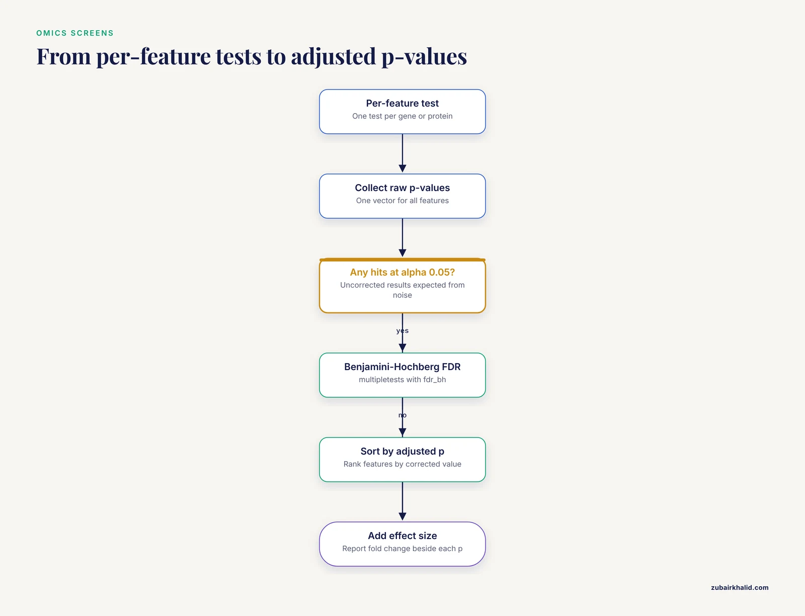
Differential expression, proteomics, and screens test thousands of features simultaneously, and at that scale raw p-values guarantee false positives. If you test 10,000 genes at alpha 0.05 with no correction, you expect roughly 500 significant results from noise alone. The false discovery rate (FDR) is the expected fraction of false positives among your declared hits, and the Benjamini-Hochberg procedure controls it by adjusting each p-value upward in proportion to its rank.
A 2D gel electrophoresis study (a proteomics method that separates proteins by charge and size) of cystic echinococcosis compared sera from eight patients against three controls, detected 263 protein spots with altered expression, reported 45 up-regulated spots with fold change of at least 2, of which 10 showed a statistical difference at p < 0.05, alongside 50 down-regulated spots of which 11 were described as suppressed, and then clustered all 263 spots by correlation into two expression clusters [5]. The design shows the classic omics shape: few biological replicates, many features, and a pipeline that combines effect size (fold change), significance, and unsupervised clustering rather than leaning on any single number.
from statsmodels.stats.multitest import multipletests

reject, p_adj, _, _ = multipletests(raw_pvalues, alpha=0.05, method="fdr_bh")
RNA-seq count data adds a dedicated modeling layer (negative binomial models in tools such as DESeq2 and edgeR), but the resulting p-values still flow through the same multiple-testing correction.
Comparing Models and Classifiers
When two classifiers score the same test set, their per-sample correctness outcomes are paired binary data, and the right test is McNemar's test. It uses only the discordant pairs, the samples where exactly one model was correct, and asks whether the disagreements are balanced.
A comparison of benign versus malignant breast lesion classification on 895 ultrasound images, spanning seven traditional machine learning models, a convolutional neural network, and an automated cloud model, used Cochran's Q test for the overall comparison across all models and the McNemar test as the pairwise post-hoc follow-up [6]. Cochran's Q is the three-or-more-model generalization of McNemar, just as Kruskal-Wallis generalizes Mann-Whitney.
from statsmodels.stats.contingency_tables import mcnemar, cochrans_q

# [[both correct,  model A right and model B wrong],
#  [model A wrong and model B right, both wrong]]
table = [[812, 30],
         [55,  98]]
res = mcnemar(table, exact=True)
Cross-validation belongs in the same decision. Comparing models on a single train-test split confuses model skill with split luck. K-fold cross-validation, which rotates the held-out portion across k partitions, gives every sample a turn in the test set and produces the paired predictions these tests need.
Comparing Tree Topologies
Phylogenetic hypothesis testing compares competing tree topologies, the branching arrangements inferred from the same sequence alignment. The Robinson-Foulds distance counts how many internal splits differ between two trees, and likelihood-based topology tests (Kishino-Hasegawa, Shimodaira-Hasegawa, and the approximately unbiased test) ask whether a candidate tree is significantly worse than the best one. A Python pipeline published for automated phylogenetic analysis unifies sequence collection, alignment with MAFFT, MUSCLE, or ClustalW, tree construction by neighbor-joining, UPGMA, maximum likelihood, or maximum parsimony, and comparative evaluation with Robinson-Foulds distances and AU, KH, and SH hypothesis tests [2]. These topology tests are standard phylogenetic tools, and the cited pipeline shows them running inside a single Python workflow instead of a chain of separate programs.
Python for Bioinformatics: Where Each Test Lives
scipy.stats and statsmodels
scipy.stats carries the standard tests: ttest_ind, ttest_rel, mannwhitneyu, wilcoxon, f_oneway, kruskal, chi2_contingency, fisher_exact, pearsonr, spearmanr, shapiro, and levene. statsmodels carries everything scipy leaves out: multipletests for FDR and family-wise corrections, pairwise_tukeyhsd for post-hoc comparisons, the contingency_tables module with mcnemar and cochrans_q, regression with per-coefficient t-tests, and the power module for sample-size planning. Pingouin wraps most of the same tests and returns effect sizes and assumption checks in the same call, which shortens the distance between running a test and reporting it properly.
scikit-learn and Cross-Validation
Model comparison lives in scikit-learn, whose cross-validation utilities are the standard way to generate the paired per-sample predictions that McNemar and Cochran's Q require. The pattern scales to genomics. DAPCy, a Python implementation of the discriminant analysis of principal components method for population genetic structure (a technique combining principal component analysis with linear discriminant analysis to describe genetic clusters), builds on scikit-learn, uses compressed sparse matrices and truncated singular value decomposition for dimensionality reduction, and evaluates with training-test cross-validation. It processes genomic datasets with thousands of samples and features in less time and with less memory than the original R implementation, which it benchmarked on Plasmodium falciparum data from MalariaGEN and on the 1000 Genomes Project [7].
Biopython for Sequences, scipy for Statistics
If you have followed any Biopython tutorial, you already know its strengths: parsing FASTA and GenBank files with Bio.SeqIO, handling alignments with Bio.AlignIO, and reading, writing, and drawing trees with Bio.Phylo. Biopython is deliberately not a statistics package. The standard pattern is to let Biopython produce the numbers and let scipy or statsmodels test them:
from Bio import SeqIO
from scipy import stats

lengths = [len(rec.seq) for rec in SeqIO.parse("contigs.fasta", "fasta")]
print(stats.describe(lengths))
print(stats.shapiro(lengths))
The same handoff pattern appears across the Python scientific stack. PyCoM, a Python library for residue-residue coevolution analysis (the study of correlated mutation positions in proteins), gives researchers query access to alignments and coevolution matrices for 457,622 proteins from UniProtKB/Swiss-Prot with lengths up to 500 residues, built explicitly so that statistical analyses of coevolution patterns can be developed on top of it [8]. And when a domain needs statistical machinery that matured elsewhere, Python connects to it: the HDX-Analyzer package for hydrogen-deuterium exchange mass spectrometry (a method that probes protein structural dynamics by measuring deuterium uptake at the backbone) pairs a Python data-processing module with an R statistical module through the rpy2 bridge [9].
Worked Scenarios
Scenario 1: Gene Expression Between Two Conditions
A molecular study of long noncoding RNA in alcohol use disorder measured GAS5 and miR-136-5p expression by reverse transcription quantitative PCR in patient tissue samples and in cell lines [10]. That two-group, continuous-outcome design is one of the most common in molecular biology, and it is small enough that the nonparametric option deserves respect.
import numpy as np
from scipy import stats

control = np.array([5.12, 5.30, 4.95, 5.61, 5.20, 5.05])   # delta-Ct values
treated = np.array([4.21, 4.40, 3.94, 4.63, 4.12, 4.35])   # delta-Ct, the normalized qPCR quantity

print(stats.shapiro(control).pvalue, stats.shapiro(treated).pvalue)

welch = stats.ttest_ind(treated, control, equal_var=False)
rank  = stats.mannwhitneyu(treated, control, alternative="two-sided")
With six samples per group, the Shapiro-Wilk test will rarely reject anything, so many analysts pre-specify the Mann-Whitney test for qPCR comparisons and report the mean difference with a confidence interval alongside it. If both tests agree, the conclusion is sturdy. If they disagree, the distribution shape, usually an outlier, is the story.
Scenario 2: Paired Measurements on the Same Units
Any before-and-after or two-systems-same-samples design follows the same recipe: compute the per-unit differences, then test those differences.
diffs = np.asarray(plan_a) - np.asarray(plan_b)
print(stats.shapiro(diffs).pvalue)

res_t = stats.ttest_rel(plan_a, plan_b)   # differences roughly normal
res_w = stats.wilcoxon(plan_a, plan_b)    # differences skewed or outliers present
The paired plan-comparison studies described above are the template. Test the differences, not the two conditions as if they were unrelated groups, and report every comparison you ran, not only the flattering ones.
Scenario 3: Two Classifiers on One Test Set
from statsmodels.stats.contingency_tables import mcnemar

# rows: model A correct, model A wrong. columns: model B correct, model B wrong
table = [[812, 30],
         [55,  98]]
res = mcnemar(table, exact=True)
print(res.statistic, res.pvalue)
Only the off-diagonal cells (30 and 55) contribute to the test. If model A wins 30 samples and loses 55, the exact McNemar test tells you whether that imbalance is plausible if the two models are equally skilled. Build the table from cross-validated predictions on the same folds, never from two different splits.
Scenario 4: Differential Signal Across Hundreds of Features
Run the per-feature test first, then pass one vector of raw p-values into the FDR correction:
import numpy as np
from scipy import stats
from statsmodels.stats.multitest import multipletests

pvals = np.array([
    stats.mannwhitneyu(omics[i, case_mask], omics[i, ~case_mask]).pvalue
    for i in range(omics.shape)
])
reject, p_adj, _, _ = multipletests(pvals, alpha=0.05, method="fdr_bh")
Sort the results by adjusted p-value, but report fold change or another effect size next to them, because with enough features even tiny effects can reach significance when measurement variance is low.
Parametric and Nonparametric Options: Pros and Cons
| Criterion | Parametric tests (Welch t, ANOVA, Pearson) | Nonparametric tests (Mann-Whitney, Wilcoxon, Kruskal-Wallis, Spearman) |
|---|---|---|
| Assumptions | Approximate normality, defined variances | Few, mostly independence |
| Power when assumptions hold | Higher | Moderately lower |
| Behavior with outliers | Sensitive, one extreme value can move the mean | Robust, ranks absorb outliers |
| Small samples | Risky unless normality is plausible | Practical default in small validation sets |
| What you estimate | Means and mean differences with confidence intervals | Ranks, medians with shape caveats, probability of superiority |
| Covariates and factorial designs | Straightforward through regression and ANOVA | Limited, specialized methods required |
| Interpretation risk | Outlier-driven means | Overclaiming about medians when shapes differ |
When the assumptions genuinely hold, parametric tests win on power, on interpretability, and on extensibility to covariates and multi-factor designs. When the assumptions fail or the sample is small, nonparametric tests win on robustness, and the power you give up is usually modest. The asymmetry matters: switching to the rank-based test costs you a little power, while staying parametric with violated assumptions can hand you a wrong answer with a confident-looking p-value attached. That asymmetry is why small-qPCR-style studies default to rank tests, and why large, well-behaved datasets default to Welch, ANOVA, and Pearson.
Common Mistakes and Limitations
- Pseudoreplication. Treating technical replicates (repeated measurements of the same biological sample) as independent observations inflates the effective sample size and produces spectacularly small p-values for nothing. Average technical replicates per biological unit before testing, or use a mixed model if you must keep them separate.
- Skipping multiple-testing correction. Any omics-scale screen without FDR control mostly reports noise. Correct at the feature level and name the correction method in your methods section.
- Trusting small-table p-values. A simulation of 2,000 random 2x2 contingency tables with cell counts from 20 to 480, all of them significant at p < 0.05 by Fisher's exact test, showed that the fragility index (how many outcome changes it takes to destroy significance) and the relative risk index (how far the observed risk sits from equivalence) capture information the p-value alone does not [11]. In small tables, significance can flip with a handful of outcome changes, so report the effect size and its confidence interval next to every p-value.
- Assuming preprocessing is neutral. A systematic comparison built 96 decision trees across 2 algorithms, 3 clinical datasets, 4 preprocessing schemes, and 2 balancing settings, and the processing choices changed model performance enough to require formal significance testing of the schemes themselves [12]. Your test result is conditional on every processing step that came before it, so report standardization, normalization, filtering, and balancing decisions with the same care as the test itself.
- Trusting the software instead of the design. The HDX-Analyzer authors observed that most software for hydrogen-deuterium exchange mass spectrometry at the time lacked proper, explicit statistical treatment [9]. A tool that prints a p-value is not a tool that chose the right test. The analyst owns that choice, whatever the language and whatever the package.
- Normality rituals on tiny samples. Running Shapiro-Wilk on five values per group and treating p > 0.05 as a certificate of normality is reading tea leaves. At small n, prefer the rank-based test or justify normality from the known behavior of the measurement.
- Reporting p-values without effect sizes. A p-value says nothing about magnitude. Pair every test with Cohen's d, r, fold change, an odds ratio, or a mean difference with a confidence interval.
One limitation deserves its own sentence: a decision table narrows the options, but the final call on a specific dataset belongs to someone who knows both the experiment and the statistics, and complex designs deserve a biostatistician's review before publication.
Frequently Asked Questions
Which statistical test should I use for my bioinformatics data in Python?
Classify your outcome as continuous or categorical, decide whether observations are independent or paired, and check whether normality is plausible. Those three answers select a row in the master table above, and scipy.stats plus statsmodels implement every test on it.
Should I use a t-test or the Mann-Whitney U test?
Use Welch's t-test when the outcome is continuous, roughly normal, and free of extreme outliers, and use the Mann-Whitney U test when the data are skewed, ordinal, or based on few observations. At small sample sizes where normality cannot be verified, the rank-based test is the safer default.
How do I correct for multiple testing in Python?
Run your per-feature test first, then pass the vector of raw p-values to statsmodels.stats.multitest.multipletests with method="fdr_bh". The Benjamini-Hochberg procedure controls the expected fraction of false positives among your declared hits, which is the standard for omics screens.
What test compares two machine learning models fairly?
McNemar's test on the paired correct-or-wrong outcomes of both models over the same test samples. For three or more models on the same samples, start with Cochran's Q and follow with pairwise McNemar tests.
Does Biopython perform statistical tests?
No. Biopython handles sequences, alignments, and phylogenetic trees. Parse and compute with Biopython, then hand the numeric summaries to scipy.stats or statsmodels for hypothesis testing.
How many samples do I need per group?
Run a power analysis before collecting data, using your expected effect size, your alpha, and your target power. Published two-group comparisons commonly plan for 80 percent power at alpha 0.05, and statsmodels.stats.power computes the required sample size from those inputs.
Sources
- Text Mining for Translational Bioinformatics
- A python-based automated pipeline for phylogenetic tree construction, visualization, and comparative statistical evaluation.
- Evaluation of Hybrid Arc and Volumetric-Modulated Arc Therapy Treatment Plans for Fractionated Stereotactic Intracranial Radiotherapy
- A decision support system for multi-target disease diagnosis: A bioinformatics approach
- Proteome evaluation of human cystic echinococcosis sera using two dimensional gel electrophoresis
- Evaluation of the performance of traditional machine learning algorithms, convolutional neural network and AutoML Vision in ultrasound breast lesions classification: a comparative study.
- DAPCy: a Python package for the discriminant analysis of principal components method for population genetic analyses.
- PyCoM: a python library for large-scale analysis of residue-residue coevolution data.
- HDX-Analyzer: a novel package for statistical analysis of protein structure dynamics
- m6A-modified lncRNA GAS5 promotes M1-polarization of microglia in alcohol use disorder.
- Statistical Significance Versus Clinical Relevance: A Head-to-Head Comparison of the Fragility Index and Relative Risk Index
- Comparison and analysis of applications of ID3, CART decision tree models and neural network model in medical diagnosis and prognosis evaluation