StringTie vs Cufflinks: Which Transcript Assembly Tool Should You Use?
By Dr. Zubair Khalid, DVM, MS, PhD ·
StringTie and Cufflinks both reconstruct transcripts from RNA-seq reads aligned to a genome, but StringTie uses a network flow algorithm that published benchmarks show is faster and produces more complete and more accurate assemblies than Cufflinks. For any new RNA-seq project, use StringTie. Reach for Cufflinks only when you need to reproduce a legacy analysis exactly or when a collaborator or journal protocol was built around the classic TopHat-Cufflinks workflow.
That is the short answer. The rest of this article explains where each tool came from, how the algorithms differ, what the benchmarks actually measured, how the downstream differential expression routes differ, and how to decide in specific situations. If you are starting to learn bioinformatics, this comparison is also a useful case study in how sequencing methods evolve: Cufflinks defined the transcript assembly problem in 2010, and StringTie solved the same problem with a better algorithm five years later.
What Transcript Assembly Actually Does
Before comparing the two tools, it helps to be precise about the problem they solve. An RNA-seq experiment shreds millions of RNA molecules into short sequencing reads, typically 50 to 150 bases each. Most reads are far shorter than the transcripts they came from, and because eukaryotic genes contain introns, reads from different isoforms of the same gene are fragmented and intermingled.
Transcript assembly is the computational step that puts those fragments back together. The assembler takes a BAM file of reads aligned to a reference genome (a BAM file is the standard compressed binary format for alignments, produced by an aligner such as HISAT2 or STAR) and infers the set of transcripts that best explains the observed read coverage and splice junctions. Each inferred transcript is a predicted isoform, meaning one of possibly several RNA molecules produced from the same gene locus by alternative splicing.
Two assembly modes exist, and both tools support a version of each:
- Reference-guided assembly. The assembler receives a gene annotation file, usually in GTF or GFF3 format, and uses it to constrain or seed transcript reconstruction. Known exons and junctions are recovered reliably, and reads outside the annotation can still suggest novel transcripts.
- De novo assembly within a genome-guided framework. The assembler ignores (or only optionally consults) the annotation and builds transcripts purely from the read alignment. This can discover genes and isoforms missing from the annotation, at the cost of more false positives.
The assembler also estimates expression, typically as TPM (transcripts per million, a normalized abundance measure that allows comparison across samples) or FPKM (fragments per kilobase of transcript per million mapped reads, an older normalization still used by both tools internally).
A note on terminology you will see throughout: both Cufflinks and StringTie are genome-guided assemblers, not pure de novo assemblers like Trinity. They need a reference genome and an alignment. That distinction matters because the choice of aligner is part of the decision, as you will see in the pipeline comparisons below.
How Cufflinks Works
Cufflinks, published in 2010 by the laboratory that also produced TopHat and Bowtie, was the first widely adopted tool for reference-guided transcript assembly and quantification from RNA-seq. It became the default second half of the TopHat-Cufflinks pipeline that thousands of papers used through the 2010s.
The core idea in Cufflinks is parsimony. It builds a splice graph from the aligned reads, where nodes represent exonic segments and edges represent possible splice junctions, and then searches for the minimum set of transcripts that explains all the observed reads. This "minimum" philosophy was designed to avoid overpredicting isoforms in an era when RNA-seq libraries were shallower and read lengths were shorter. The trade-off is that when two isoforms share most of their exons, the parsimony filter can merge them or drop the lower-abundance one, so recall of closely related isoforms suffers at coverage levels that modern projects routinely generate.
Cufflinks ships as a suite. The typical legacy workflow looks like this:
- Align reads with TopHat, a splice-aware aligner built on Bowtie.
- Assemble transcripts for each sample with
cufflinks. - Merge per-sample assemblies into a consistent transcript set with
cuffmerge, which can also consult a reference annotation. - Estimate abundance across all samples with
cuffquantand test for differential expression and differential splicing withcuffdiff.
Cuffdiff performs statistical testing directly on FPKM values using a model of the library and a beta distribution for transcript-level variability. This design choice, testing on normalized abundances rather than raw counts, became a major point of criticism in later years, because count-based tools such as DESeq2 and edgeR model the sampling noise of RNA-seq counts more faithfully. Many groups that used Cuffdiff on very shallow data reported inflated numbers of significant calls, a problem documented in the differential expression literature and one reason the field moved to count-based testing. This is established knowledge in the field rather than a single-study claim, and it is one of the strongest practical arguments against starting a new project on the Cufflinks stack today.
How StringTie Works
StringTie, published in Nature Biotechnology in 2015 by the Salzberg laboratory at Johns Hopkins (the same group behind HISAT2 and Bowtie), reframed transcript assembly as a network flow problem [1]. In this framing, read coverage entering and leaving each node of the splice graph behaves like flow in a network, and the assembler searches for a set of transcripts whose predicted coverage profiles match the observed flow as closely as possible.
The practical consequence of the network flow approach is that StringTie does not insist on a minimal transcript set. Instead it explicitly balances coverage across candidate transcripts, which lets it recover low-abundance isoforms that a parsimony filter would discard, and it produces assemblies that track the data more closely. StringTie also combines the network flow step with optional de novo assembly of unannotated regions, so a single run can both recover annotated transcripts and propose novel ones [1].
Two design features of StringTie matter enormously in practice:
- Native annotation-awareness without a separate merge step per sample. StringTie can assemble every sample independently and then run a dedicated merge mode that produces a consensus transcript set across all samples, analogous to what cuffmerge does but integrated and faster.
- Quantification mode for known transcripts. With its estimation mode (the
-eflag), StringTie skips assembly and only estimates abundances for transcripts in a supplied reference, which is exactly what you want for differential expression on a well-annotated genome. Combined with the-Bflag it writes the tables that the Ballgown R package reads directly.
StringTie outputs standard GTF, so its assemblies feed into any downstream tool that consumes GTF, including gffcompare for comparing assemblies against annotations and featureCounts or the StringTie prepDE script for generating count matrices.
Side-by-Side Comparison Table
This table is the core of the comparison. Read it as a summary of everything developed in the sections that follow.
| Feature | Cufflinks | StringTie |
|---|---|---|
| First released | 2010 | 2015 |
| Core algorithm | Parsimony-based minimal transcript set from a splice graph | Network flow (maximum flow) algorithm with optional de novo assembly [1] |
| Assembly modes | Reference-guided, de novo within genome guidance | Reference-guided, de novo within genome guidance [1] |
| Typical aligner pairing | TopHat (legacy), STAR | HISAT2, STAR, any splice-aware aligner |
| Merging multiple samples | Separate cuffmerge step | Built-in merge mode |
| Quantification output | FPKM per transcript and gene | TPM and coverage per transcript and gene, with optional Ballgown tables |
| Differential expression route | Cuffdiff (FPKM-based testing) | Ballgown, or export counts for DESeq2 and edgeR |
| Benchmark accuracy on human blood RNA-seq (90 million reads) | 7,187 correctly assembled transcripts | 10,990 correctly assembled transcripts, a 53% increase [1] |
| Benchmark accuracy on simulated data | 6,310 correctly assembled transcripts | 7,559 correctly assembled transcripts, a 20% increase [1] |
| Runtime | Slower on every dataset tested in the original comparison | Faster on all datasets tested against Cufflinks [1] |
| Compute demand in a six-pipeline head-to-head | Cufflinks-Cuffdiff demanded the most computing resources of the six pipelines tested [2] | Moderate, and paired pipelines scale well |
| Sensitivity profile in pipeline comparisons | Less sensitive for low-abundance genes | More sensitive to genes with low expression levels [2] |
| Maintenance status | Legacy, in maintenance mode | Actively developed, with long-read support in later versions |
| Best use today | Reproducing legacy published analyses, protocol-matched comparisons | All new assembly and quantification projects |
Two rows deserve emphasis. The accuracy numbers come from the original StringTie benchmark, which compared StringTie against Cufflinks, IsoLasso, Scripture, and Traph on both simulated and real data [1]. The compute-demand row comes from an independent 2022 comparison of six analysis pipelines on four RNA-seq datasets from mouse, human, rat, and macaque, which found that Cufflinks-Cuffdiff demanded the highest computing resources while Kallisto-Sleuth demanded the least [2]. Independent evaluation matters here. A tool author's own benchmark favors the author's tool, so the fact that separate comparison studies keep reaching conclusions consistent with the original StringTie paper is the meaningful signal.
Assembly Accuracy and Completeness: What the Benchmarks Show
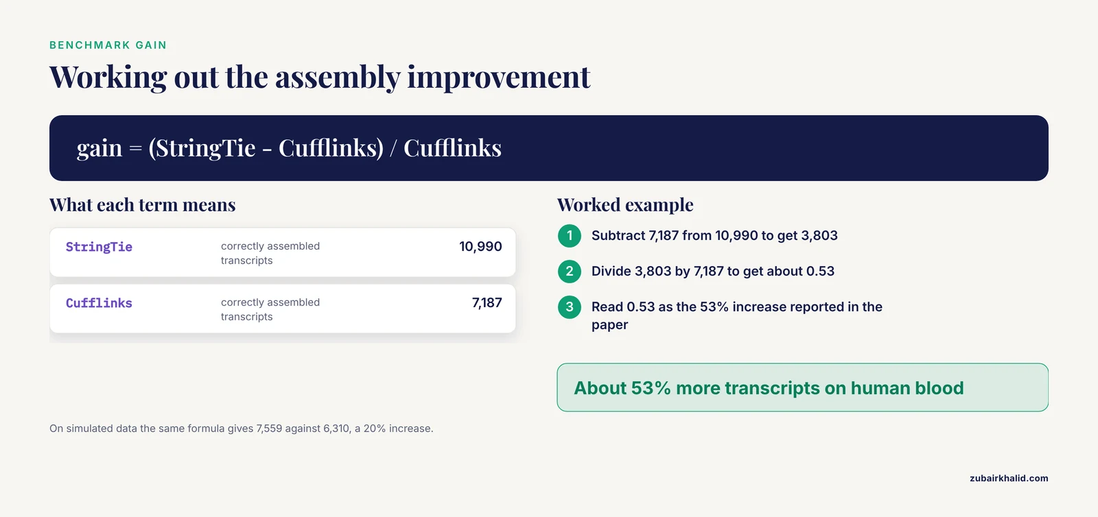
The headline numbers in the StringTie versus Cufflinks question come from the original publication. On 90 million reads from human blood, StringTie correctly assembled 10,990 transcripts while Cufflinks assembled 7,187, a 53% increase in correctly assembled transcripts [1]. On a simulated dataset, StringTie correctly assembled 7,559 transcripts against 6,310 for Cufflinks, a 20% improvement [1]. The paper also reports better expression-level estimates relative to Cufflinks, and faster runtime on every dataset tested [1].
What do "correctly assembled" and "more complete" mean in this context? Correct means the reconstructed transcript matched a known reference isoform in its exon structure. Complete means more of the true transcript population was recovered. The Cufflinks parsimony strategy, designed for cautious assembly on sparse data, systematically loses transcripts that share exons with more abundant isoforms. The network flow strategy recovers them because it distributes coverage across the full set of transcripts that could have generated the observed graph.
Two caveats keep this honest. First, these are short-read, Illumina-style benchmarks on bulk RNA-seq. Later tools have pushed the frontier further. Strawberry, a genome-guided assembler that also uses network flow for assembly but a different latent class model for quantification, outperformed both Cufflinks and StringTie in simulated assembly and quantification accuracy and showed the highest correlation with NanoString probe counts on a real dataset [3]. Second, for single-cell full-length data, specialized assemblers outperform both general tools. scRNAss, a single-cell assembler that imputes dropout events and combines splice junctions, was evaluated against StringTie, Cufflinks, and CLASS2 and showed superior recovery of novel isoforms with better computational efficiency [4]. Neither caveat changes the StringTie versus Cufflinks verdict. Both newer tools beat both of the older ones, and StringTie remains the strongest of the two options in this article for bulk short-read projects.
A third caveat concerns your own data. Benchmark differences of tens of percent in recovered transcripts matter most when your biological question involves isoform structure. If your question is purely gene-level differential expression on a well-annotated genome, the assembly accuracy differences shrink in importance, and speed, sensitivity, and downstream integration dominate the decision.
Speed and Compute Cost
Runtime and memory are not vanity metrics. A transcriptome assembly that takes eight core-hours per sample turns a 24-sample project into a week of waiting and a scheduling headache, while the same project with a faster tool finishes overnight.
The original StringTie paper reports faster runtime than Cufflinks on all datasets tested [1], and the independent six-pipeline comparison later confirmed the pattern at the pipeline level. In that study, which benchmarked six procedures on four RNA-seq datasets from mouse, human, rat, and macaque, the Cufflinks-Cuffdiff route demanded the most computing resources of any pipeline tested, while the lightweight pseudoalignment route demanded the least [2]. StringTie-based pipelines sat comfortably in the middle: fast enough for routine use on a lab server, and dramatically lighter than the full Cufflinks suite on the same data.
The practical rule this generates is simple. If you are provisioning compute for a new project, budget for HISAT2 or STAR plus StringTie, not for TopHat plus the Cufflinks suite. If you are forced to work within a Cufflinks-based protocol, plan for the longer runtime and schedule accordingly rather than discovering the bottleneck mid-project.
Differential Expression: Cuffdiff Versus the Modern Route
This is where the difference between the two tools stops being about assembly and becomes about statistics, and it is the point where the wrong choice quietly damages a paper.
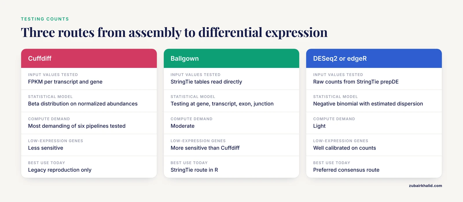
The Cufflinks route ends at Cuffdiff, which tests differential expression using FPKM values. The StringTie route offers two endpoints. The first is Ballgown, an R package built by the same team as StringTie that reads StringTie output directly and performs statistical testing at gene, transcript, exon, and junction levels. The second, and the one most analysts now prefer, is to run StringTie in estimation mode and convert its output to a raw count matrix, then hand those counts to DESeq2 or edgeR.
Why do count-based tools win? RNA-seq counts follow a negative binomial distribution whose variance depends on the mean. DESeq2 and edgeR model exactly that structure, estimate dispersion across replicates, and produce well-calibrated p-values. FPKM-based testing conflates library size, transcript length, and sampling noise into a single normalized quantity that does not map cleanly onto any standard distribution. This is textbook-level knowledge in modern RNA-seq analysis, and it explains why the field's consensus workflows moved to counts roughly a decade ago.
The 2022 six-pipeline comparison adds a useful empirical layer to this. The study found that pipelines using HTSeq for quantification produced highly correlated gene expression values, fold changes, and q-values, while the largest disagreements between pipelines appeared at genes with very high or very low expression [2]. It also found that the HISAT2-StringTie-Ballgown pipeline was more sensitive to genes with low expression levels, whereas Kallisto-Sleuth was mainly informative for medium to high abundance genes [2]. If your experiment depends on detecting subtle changes in low-abundance transcripts, immune receptors, transcription factors, and long non-coding RNAs often sit in this range, the StringTie route has a documented sensitivity advantage.
One related point deserves its own sentence: whether you use Cuffdiff or Ballgown or DESeq2, differential expression testing requires biological replicates, and no assembler choice compensates for a design with too few of them.
The Two Classic Pipelines, Side by Side
Because tool choice and aligner choice are entangled, most people actually choose between two named pipelines. A detailed plant-focused protocol in Methods in Molecular Biology describes exactly these two, HISAT-StringTie-Ballgown and TopHat-Cufflinks, step by step from raw reads through differential expression, and discusses alternative tools for each stage [5]. The protocol exists because both pipelines remain in circulation, and because plant scientists in particular still encounter published datasets processed with either one.
The pipelines stage by stage:
- TopHat-Cufflinks. TopHat aligns reads to the genome using Bowtie and identifies splice junctions from read gaps. Cufflinks assembles, cuffmerge consolidates per-sample assemblies, and cuffdiff tests differential expression.
- HISAT2-StringTie-Ballgown. HISAT2, the successor aligner from the same laboratory that developed TopHat, aligns reads with a hierarchical index of the genome and known splice sites. StringTie assembles and quantifies, and Ballgown performs statistical testing on the StringTie tables.
The second pipeline is faster at every stage, produces the more complete assembly per the benchmarks above, and connects to a statistical framework with better behavior on count data. The first pipeline survives because of reproducibility. Thousands of older datasets were processed with it, and reanalysis of legacy data sometimes requires matching the original method. A 2024 protocol that documents both pipelines in parallel reflects exactly this reality [5].
A concrete illustration of the two tools coexisting comes from a bacterial small RNA study. Researchers investigating RNase III-regulated transcripts in Streptococcus pyogenes performed differential expression analysis of RNA-seq data using both Cufflinks and StringTie, identifying intergenic regions whose expression changed after deletion of the RNase III gene, then filtered twelve differentially expressed regions down to six putative small RNAs by visual inspection in genome browsers [6]. The dual-tool approach served as an internal consistency check, a pattern that generalizes well.
When to Use StringTie
StringTie is the right choice in nearly every situation you will encounter with bulk RNA-seq on a reference genome. Specifically:
- New differential expression projects. Align with HISAT2 or STAR, assemble or estimate with StringTie, and test with Ballgown or a count-based tool. This is the current consensus route, and the sensitivity data support it for low-abundance genes [2].
- Novel isoform and long non-coding RNA discovery. The de novo-capable assembly mode and the network flow algorithm recover isoforms and intergenic transcripts that parsimony-based assembly misses [1]. Novel non-coding transcript discovery is an area where this matters a lot. Intergenic long non-coding RNA identification in wheat stripe rust resistance, for example, produced a catalog of 2,736 expressed lincRNAs from strand-specific RNA-seq, of which 515 were differentially expressed during infection, and the transcript identifiers reported carry the MSTRG prefix that StringTie's merge step generates [7]. That naming convention is a small but telltale marker of how deeply StringTie is embedded in current non-coding RNA workflows.
- Bacterial and compact genomes. The Streptococcus pyogenes small RNA study shows StringTie working in an intergenic-focused, prokaryotic context alongside Cufflinks [6]. Compact genomes amplify the benefit of accurate assembly because intergenic regions are short and the risk of merging adjacent transcription units is high.
- Large cohorts and tight compute budgets. The runtime advantage over Cufflinks is consistent across all tested datasets [1], and the pipeline-level compute data reinforce it [2].
- Teaching and training. If you are designing a bioinformatics course or working through one, learn the StringTie pipeline as your primary workflow. It is the one you will use professionally, and understanding why it replaced Cufflinks teaches you more about the underlying statistics and algorithms than memorizing either tool's flags.
When Cufflinks Still Makes Sense
Cufflinks is not wrong to use in every context. Three situations justify it:
- Exact reproduction of a published legacy analysis. If you are reanalyzing a dataset whose original publication used TopHat-Cufflinks-Cuffdiff and you need results directly comparable to the original, run the same pipeline. Mixing tools changes transcript definitions and quantification, and any difference you observe would then confound the biological comparison.
- Protocol-matched multi-lab studies. A consortium protocol that specifies Cufflinks is a protocol you follow, then note the constraint in your methods section.
- Cross-pipeline validation. Running a second, structurally different pipeline and checking that findings agree is a legitimate robustness strategy. The cumulus cell infertility study used three pipelines in parallel, STAR-Cufflinks, TopHat-HTSeq, and HISAT2-StringTie, and took the 234 differentially expressed genes consistently identified across all of them as its high-confidence set, then validated key genes by RT-qPCR [8]. The same logic applies at smaller scale: if a result survives both StringTie and Cufflinks processing, it is robust to assembler choice.
What does not justify Cufflinks is the belief that it is more accurate or more conservative in a way that protects you from errors. The benchmarks point the other way. Nostalgia and reproducibility are legitimate reasons, accuracy is not.
Worked Scenarios
Scenario 1: Standard differential expression, 6 samples, well-annotated mammalian genome. Use HISAT2 or STAR for alignment, StringTie in estimation mode against the reference annotation to produce per-transcript coverage and Ballgown tables, and run testing in Ballgown or export counts for DESeq2. Do not assemble novel transcripts for this question. The annotation is good, the question is gene-level, and estimation mode is the fastest, most reproducible path. Expect this to run in minutes to tens of minutes per sample on a normal lab server.
Scenario 2: Novel isoform discovery in a cancer cell line. Cancer transcriptomes are messy, with fusion transcripts, novel exon connections, and altered isoform usage. Assemble every sample de novo-capable with StringTie and the reference annotation provided for guidance, merge all per-sample GTF files with StringTie's merge mode to get a consistent transcript catalog, then compare the merged assembly to the reference with gffcompare to classify each transcript as known, novel isoform of a known gene, or intergenic novel. Validate candidates at the sequence level before claiming novelty. This is the scenario where the 53% assembly improvement over Cufflinks translates most directly into biology [1].
Scenario 3: Searching for small RNAs in a bacterial genome. Follow the logic of the Streptococcus pyogenes study. Align strand-aware reads, run differential analysis over intergenic regions using StringTie (optionally with Cufflinks as a second opinion), rank regions by fold change and significance, and inspect surviving candidates in a genome browser to remove artifacts before experimental validation [6]. In that study, twelve regions passed the initial statistical filter and six survived visual verification [6], a reminder that computational candidate lists are hypotheses, not discoveries.
Scenario 4: Reanalyzing someone else's legacy dataset. First check the original methods. If the paper used Cufflinks and you need gene-level differential expression comparable to the original, decide deliberately: exact reproduction means Cufflinks, modernization means StringTie plus DESeq2 with a clear statement that absolute values are not comparable to the original paper. Both choices are defensible. Silence about which you did is not.
Scenario 5: Confirming a result is not an assembler artifact. Run your two or three best pipelines in parallel, as the cumulus cell study did with STAR-Cufflinks, TopHat-HTSeq, and HISAT2-StringTie [8], and take the intersection. Budget extra compute for the Cufflinks arm, because it is the expensive one [2].
Scenario 6: Building a teaching module. If you are putting together material for a bioinformatics course, teach StringTie as the primary assembler, include a short section on Cufflinks history so students can read older papers literately, and use the network flow versus parsimony contrast as a worked example of how algorithmic choices in genomics get evaluated and replaced.
Practical Command Walkthrough
The following commands show a minimal HISAT2-StringTie workflow for one sample. They assume a prebuilt HISAT2 genome index named GRCh38, a reference annotation genes.gtf, and paired-end FASTQ files.
hisat2 -p 8 -x GRCh38 -1 sample_R1.fq.gz -2 sample_R2.fq.gz | samtools sort -o sample.sorted.bam
stringtie sample.sorted.bam -G genes.gtf -o sample.gtf -A sample_gene_abundance.tsv
The first line aligns reads and produces a coordinate-sorted BAM. The second line assembles transcripts guided by the annotation and writes a GTF plus a gene-level abundance table. Run both lines once per sample.
After all per-sample GTF files exist, run StringTie in merge mode over the list of per-sample GTFs to produce a consensus assembly, optionally anchored to the reference annotation. Then estimate abundances against that merged assembly in estimation mode with the Ballgown output flag enabled:
stringtie -e -B -G merged.gtf -o sample_est.gtf sample.sorted.bamThis produces the folder of tables that Ballgown reads directly in R. For DESeq2 or edgeR, generate a count matrix from the estimation-mode GTF files using the StringTie prepDE script instead.
The equivalent legacy steps with Cufflinks would be cufflinks on each sorted BAM, cuffmerge across the assemblies, and cuffdiff across conditions. The commands themselves are straightforward and remain documented. The issues are runtime, the FPKM-based statistics, and the sensitivity profile described above.
Common Mistakes and Limitations
These are the errors that show up repeatedly in real projects and review comments.
- Mixing assemblers across samples within one comparison. Assembling some samples with StringTie and others with Cufflinks produces transcript sets that do not correspond, and downstream merging papers over noncomparable definitions. Pick one assembler per project and apply it to every sample.
- Testing differential expression on FPKM or TPM directly. Normalized abundances are for reporting and visualization. Statistical testing on counts with DESeq2, edgeR, or a well-specified model in Ballgown gives better-calibrated results. The empirical evidence that pipeline choice shifts expression values most strongly at high and low abundance genes [2] makes this worse, not better, for the transcripts you care about most.
- Trusting a single assembler's novel transcript list. Novel isoform predictions include false positives from read mapping errors, incomplete splice junction evidence, and artifacts. Filter by expression support, inspect in a genome browser as the bacterial sRNA study did [6], and require replicate consistency before experimental follow-up.
- Forgetting strand specificity. If your library is stranded, tell the aligner and assembler. Unstranded settings on stranded data create antisense phantom transcripts, and both Cufflinks and StringTie will faithfully assemble garbage you fed them.
- Assuming benchmark rankings transfer to every data type. The headline comparisons are bulk short-read results. For single-cell full-length data, purpose-built assemblers beat both tools [4]. For long-read platforms, use tools designed for long reads. Matching the tool class to the data type is part of the decision.
- Underestimating Cuffdiff compute and runtime. In a head-to-head of six pipelines, Cufflinks-Cuffdiff was the most demanding [2]. Plan for it if legacy reproduction forces the choice.
- Treating MSTRG identifiers as gene IDs. StringTie merge assigns its own loci names, as seen in published non-coding RNA catalogs [7]. Map merged transcript IDs back to gene symbols before enrichment analysis, or your gene set tests will silently drop transcripts.
- Ignoring newer tools entirely. Strawberry outperformed both Cufflinks and StringTie in simulated assembly and quantification accuracy and correlated best with NanoString counts on real data [3]. For a project where isoform quantification accuracy is the whole point, evaluating it alongside StringTie is reasonable. Staying on Cufflinks because it was the default in 2013 is not.
One general limitation frames all of the above: assembly quality depends jointly on the assembler, the aligner, read depth, fragment length distribution, and library strandedness. No tool choice fixes a poorly designed library or an underpowered comparison, and interpreting transcript-level results for individual genes requires domain-specific follow-up validation.
Frequently Asked Questions
Is StringTie simply better than Cufflinks for RNA-seq?
For new projects, yes. Benchmarks show StringTie assembles more transcripts correctly, estimates expression at least as accurately, and runs faster than Cufflinks [1]. Cufflinks remains appropriate only for reproducing legacy analyses or satisfying a fixed protocol [5].
What is the main algorithmic difference between StringTie and Cufflinks?
Cufflinks seeks the minimal set of transcripts that explains the reads, which can drop low-abundance isoforms. StringTie treats coverage as flow through a splice graph and solves a network flow problem, recovering more complete assemblies including low-abundance isoforms [1].
Can I run both StringTie and Cufflinks on the same data?
Yes, and it is a legitimate validation strategy. A Streptococcus pyogenes small RNA study ran differential analysis with both tools and cross-checked candidate intergenic transcripts in a genome browser [6], and a cumulus cell study ran three pipelines in parallel and took the consistently identified differentially expressed genes as its high-confidence set [8].
Do StringTie and Cufflinks need a reference annotation?
Both can assemble from the genome alignment alone, but both perform better with an annotation file guiding assembly, and StringTie's estimation mode is specifically designed for quantifying annotated transcripts. For novel transcript discovery, provide the annotation for comparison but let assembly run beyond it.
Which tool should I use for differential expression?
Use StringTie with Ballgown, or better, export StringTie counts to DESeq2 or edgeR. Cuffdiff tests FPKM values rather than counts and was the most compute-hungry pipeline in a six-way comparison, while the StringTie route showed greater sensitivity for low-expression genes [2].
Is Cufflinks obsolete?
Functionally, mostly. It is in maintenance mode, it is slower, and its assembly and statistical methods have been superseded. Its remaining role is reproducibility of older published analyses, and protocols documenting both pipelines side by side reflect that legacy status rather than scientific parity [5].
Sources
- StringTie enables improved reconstruction of a transcriptome from RNA-seq reads.
- A comparison of transcriptome analysis methods with reference genome.
- Strawberry: Fast and accurate genome-guided transcript reconstruction and quantification from RNA-Seq.
- scRNAss: a single-cell RNA-seq assembler via imputing dropouts and combing junctions.
- Plant Transcriptome Analysis with HISAT-StringTie-Ballgown and TopHat-Cufflinks Pipelines.
- Identification of streptococcal small RNAs that are putative targets of RNase III through bioinformatics analysis of RNA sequencing data.
- Identification and expression analysis of intergenic long non-coding RNAs (lincRNA) associated with stripe rust resistance in wheat.
- RNA-Seq Analysis of Human Cumulus Cells Identifies Angiogenic Pathways Associated with Infertility.