Spike-in Normalization for RNA-seq
By Dr. Zubair Khalid, DVM, MS, PhD ·

By the end of this guide you will be able to decide whether your RNA-seq experiment needs spike-in normalization, design the spike-in addition so it measures the right quantity, compute spike-in-based size factors in R, and troubleshoot the errors that quietly destroy fold changes. You will also know when to stay with TMM or DESeq2 normalization instead, and how to check that choice on your own data.
Have the following on hand: R 4.3 or newer with the Bioconductor packages edgeR, DESeq2, tximport, scran, and RUVSeq, plus Salmon and featureCounts on your command line. On the wet-lab side you need a validated ERCC spike-in mix and the manufacturer's analyte table listing the expected concentration of each control transcript.
Spike-in normalization for RNA-seq answers a question that ordinary between-sample normalization cannot: how did the absolute amount of each transcript change, rather than how did its share of the sequencing library change? A spike-in is a synthetic RNA molecule of known sequence and known concentration added to every sample in a fixed amount. Because the input is known, spike-in reads act as an external ruler for sequencing depth and processing efficiency. Relative methods such as TMM estimate their scaling factors from the endogenous genes and assume most genes do not change, an assumption that fails under global transcriptional shifts, and Robinson and Oshlack demonstrated how strongly normalization choices shape differential expression results [1].
What Spike-ins Are and Why RNA-seq Needs Them
The most widely used controls come from the External RNA Control Consortium (ERCC), a set of 92 synthetic polyadenylated RNA transcripts distributed in two mixes whose concentrations span several orders of magnitude. Each transcript carries a sequence absent from most model genomes, so aligners and pseudoaligners count it separately from endogenous genes without ambiguity.
Every read count is the product of three terms: the number of transcript molecules in the sample, the sequencing depth, and a chain of technical efficiencies spanning extraction, fragmentation, reverse transcription, and amplification. Normalization divides out depth and efficiency so counts reflect molecules. Relative methods such as TMM (trimmed mean of M values) and RLE (relative log expression, the median-of-ratios method inside DESeq2) estimate those nuisance factors from the endogenous genes themselves. That works only while the assumptions hold: most genes are not differentially expressed, and total RNA output is roughly constant across samples. Evans, Hardin, and Stoebel provide the standard account of these assumptions and of the inflated false positives that follow when they break [2].
The failure mode is compositional. If a treatment doubles transcription across half the transcriptome, a relative method sees the unchanged half as downregulated because its share of the library shrank, even though nothing about those genes changed in absolute terms. Spike-ins break the circularity by supplying a fixed external reference, so the scaling factor comes from molecules of known input rather than from the shifting transcriptome itself.
The arithmetic is simple. The spike-in size factor for a sample is its spike-in read total, rescaled so the factors across samples average to one. Dividing every count in that sample by its factor places all samples on a common absolute scale, the same algebra DESeq2 applies with its median-of-ratios factors, with ERCC totals substituted for endogenous ones.
Spike-ins do not correct everything. They have their own lengths, no introns, and their own capture efficiencies, so they calibrate scale rather than per-gene biases such as GC content or transcript length. Those biases belong to the quantification step, for example the sequence and GC bias correction in Salmon, or to downstream conditional methods. Think of spike-ins as a ruler for how much RNA survived the pipeline, not as a per-gene error correction device.
When Spike-in Normalization Helps, and When It Backfires
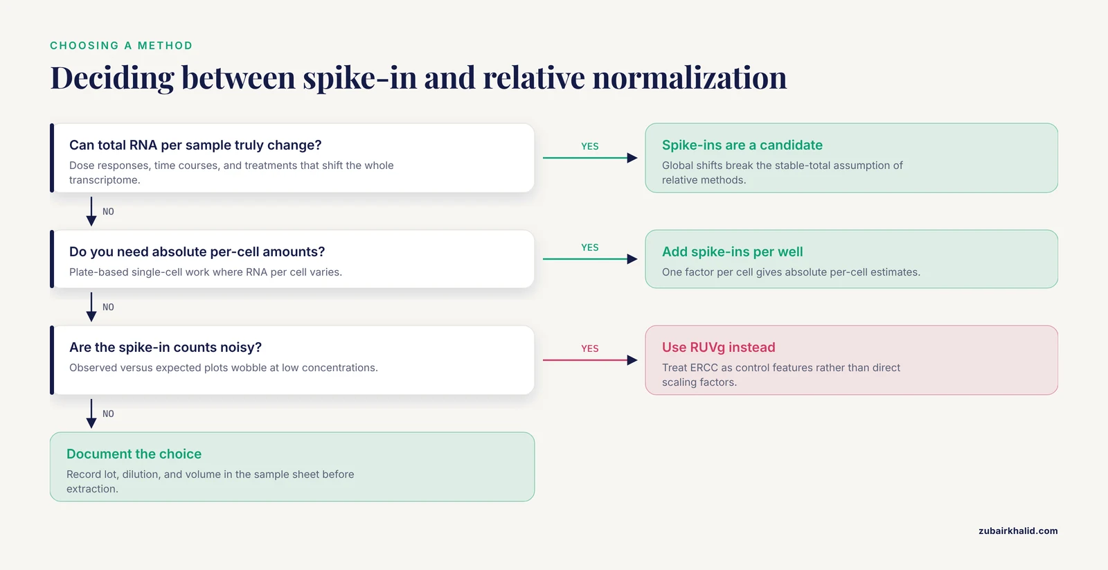
The clearest wins come from experiments with genuine global shifts. Wang and colleagues profiled cancer cells treated with paclitaxel, celecoxib, and the combination using single-cell RNA-seq. Normalizing endogenous genes to spike-in molecules showed that cellular mRNA abundance itself was dynamically regulated, and a random forest model classified single cells into transcriptional repression, amplification, and control-like states, with the drug combination driving amplification of mitochondrial oxidative phosphorylation genes linked to stronger cell killing [3]. A relative method would have forced total RNA per cell to look constant and erased the headline result. A correction to that article was later published, so consult the corrected version before quoting exact effect sizes [4].
Single-cell RNA-seq (scRNA-seq) is the other natural home for spike-ins, because total RNA per cell varies with cell cycle, treatment, and cell type. In an assessment of seven normalization methods on single-cell data generated from diluted RNA samples, methods that used ERCC spike-ins significantly outperformed methods that did not [5]. Wider surveys agree that the best method depends on the data type and on the information available [6]. Practice has also moved on. A 2025 benchmark of six widely used single-cell methods found Dino strongest for clustering 10x Genomics data, scTransform strongest for full-length library protocols, and SCnorm suitable for small datasets, none of which require spike-ins [7]. Spike-ins are not mandatory in single-cell analysis, but they remain the only route to absolute per-cell questions when you need to ask them.
In bulk RNA-seq the same logic applies to dose responses, time courses, developmental series, and tissue comparisons where cell composition differs. Any design where the whole transcriptome moving is a plausible outcome is a candidate for spike-ins, because relative methods redistribute that signal across unchanged genes.
Spike-ins backfire when used carelessly. Risso and colleagues evaluated ERCC controls directly and found them not reliable enough to drive standard global-scaling or regression-based normalization, because spike-in measurements carry their own technical noise, especially at low concentrations [8]. Their alternative, remove unwanted variation (RUV), treats spike-ins as control features in a factor analysis and adjusts endogenous genes for the estimated unwanted factors. The distinction matters in practice: spike-ins are excellent as an external scale reference and as control features, and risky as the sole basis for a regression model.
A related caution applies to benchmarking your pipeline. Differential expression methods evaluated on spike-in datasets generated from one bulk RNA sample measure technical variability only, which makes those test results less reliable than benchmarks that include biological variation, and method rankings can differ sharply between the two settings [9].
Designing the Wet-Lab Side of Spike-in Normalization
What the spike-ins measure depends entirely on where you add them, and this is the most consequential design decision in the whole workflow.
- Added to the lysis buffer before RNA extraction, with a constant number of cells per sample, spike-ins track losses through extraction, fragmentation, and library construction, and report absolute RNA per fixed biological input.
- Added to purified RNA after you have already loaded equal masses, spike-ins track library preparation only, because mass loading has already removed total RNA differences from the comparison.
- Added at a constant amount per cell or per well in single-cell experiments, spike-ins enable absolute per-cell estimates, the design behind the transcriptional amplification findings above [3].
Whichever design you choose, the operating rules are the same. Use one lot of one mix for the entire study. Prepare a single master dilution, aliquot it, and add the same volume to every sample across every batch, lane, and operator. Randomize conditions across processing batches so the spike-in reference is shared rather than confounded with treatment. Never tune the spike-in amount per sample to compensate for input differences, because that deletes the signal the spike-ins exist to detect. Record the lot number, dilution, and added volume in the sample sheet beside the biological metadata.
Keep the spike-in fraction small but measurable. A sliver of reads makes the size factor unstable, while a large fraction wastes sequencing on controls. Run a pilot, read the observed spike-in percentage from the alignment summary, and adjust the master dilution once, before the real experiment begins.
If you receive RNA that was already extracted without spike-ins, the absolute option is gone for the extraction step, and the methods section should say so. Adding spike-ins at that point still calibrates library preparation, which is often the dominant source of variation behind well-controlled extractions, but the result cannot be presented as absolute quantification of the original biological material.
Spike-in RNA-seq Normalization Step by Step
The walkthrough assumes bulk RNA-seq with ERCC controls added before extraction, quantified with Salmon, and tested with DESeq2 or edgeR. The same factor arithmetic applies to genome-alignment counts and to single-cell count matrices. The table summarizes the main normalization strategies and where each one belongs.
| Strategy | Reference used | Core assumption | Best for | Implementation |
|---|---|---|---|---|
| , - | , - | , - | , - | , - |
| TMM [1] | Endogenous genes | Most genes not DE, stable total RNA | Standard bulk DE | edgeR::calcNormFactors() |
| RLE | Endogenous genes | Same as TMM | Standard bulk DE | DESeq2::estimateSizeFactors() |
| Spike-in size factors | ERCC totals | Spike-ins added identically, behave like endogenous RNA | Global shifts, absolute scales | Manual formula or scran::computeSpikeFactors() |
| RUVg [8] | ERCC as control features | Unwanted variation is low dimensional | Noisy spike-ins, batch effects | RUVSeq::RUVg() |
| Endogenous scRNA models [7] | Endogenous genes | Modeled count-depth relationships | Droplet and full-length scRNA | sctransform, SCnorm, Dino |
| Upper quartile [10] | Endogenous genes | Stable expression bulk | Targeted panels such as TempO-Seq | EDASeq or limma pipelines |
Step 1: Fix the design and document it
Decide which of the three designs above matches your biological question, then freeze the spike-in lot, dilution, and volume in the sample sheet before any RNA is extracted.
Step 2: Build a reference that contains the spike-ins
The controls must be present in the sequences you index and in the annotation you count against, or they will return zero reads without any error message.
# Pseudoalignment route with Salmon
cat gencode.v44.transcripts.fa ERCC_transcripts.fa > transcripts_plus_ERCC.fa
salmon index -t transcripts_plus_ERCC.fa -i salmon_index -k 31
salmon quant -i salmon_index -l A -p 8 \
  -1 S1_R1.fastq.gz -2 S1_R2.fastq.gz \
  -o salmon/S1
# Genome alignment route, counted with featureCounts
cat GRCh38.fa ERCC_genomic.fa > genome_plus_ERCC.fa
cat gencode.v44.annotation.gtf ERCC.gtf > annotation_plus_ERCC.gtf
# Build your splice-aware index (STAR or HISAT2) from the combined files, then count:
featureCounts -T 8 -p -t exon -g gene_id \
-a annotation_plus_ERCC.gtf \
-o counts/S1.txt aligned/S1.bamTranscript and gene identifiers must match across the FASTA, the GTF, the tx2gene mapping if you use tximport, and the analyte table, for example ERCC-00002 written identically in all of them.
Step 3: Import the counts
library(tximport)
samples <- read.delim("samples.tsv")
files <- file.path("salmon", samples$sample, "quant.sf")
names(files) <- samples$sample
txi <- tximport(files, type = "salmon")
counts <- round(txi$counts)   # DESeq2 and RUVSeq want integers
With featureCounts output, read the per-sample files and cbind the gene count columns into one matrix instead. Sample identifiers in samples.tsv must match the column names of the count matrix.
Step 4: Verify the spike-ins are present
is_spike <- grepl("^ERCC-", rownames(counts))
table(is_spike)
spike_tot <- colSums(counts[is_spike, , drop = FALSE])
round(100 * spike_tot / colSums(counts), 3)
Expected output:
is_spike
FALSE  TRUE
19801    92

   S1    S2    S3    S4
0.512 0.498 0.521 0.505
Ninety-two TRUE rows confirm the full ERCC set, and a stable percentage near half a percent says the addition was consistent. Zero TRUE rows mean the reference never contained the controls, the most common silent failure in this workflow.
Step 5: Compute the spike-in size factors
stopifnot(all(spike_tot > 0))
spike_sf <- spike_tot / exp(mean(log(spike_tot)))
names(spike_sf) <- colnames(counts)
round(spike_sf, 3)
S1 S2 S3 S4
1.024 0.996 1.042 0.938Dividing each sample by its factor makes the spike-in counts equal across samples on average, and applies the same scaling to every endogenous gene. The geometric mean centering matches the DESeq2 convention, so the numbers are directly comparable to ordinary size factors. The factors also absorb sequencing depth automatically, because deeper sequencing of the same library raises endogenous and spike-in counts proportionally.
Step 6: Test differential expression with the spike-in factors
library(DESeq2)
dds <- DESeqDataSetFromMatrix(
  countData = counts,
  colData   = samples,
  design    = ~ condition
)
sizeFactors(dds) <- spike_sf
dds <- DESeq(dds)
res <- results(dds, contrast = c("condition", "treated", "control"))
head(res[order(res$padj), ], 10)
DESeq2 uses the assigned factors for normalization, dispersion estimation, and testing. In edgeR, set the library sizes to the spike-in totals, which makes counts per million equal to counts per million spike reads:
library(edgeR)
y <- DGEList(counts = counts, samples = samples)
y <- y[!is_spike, , keep.lib.sizes = FALSE]
y$samples$lib.size <- spike_tot[colnames(y)]
design <- model.matrix(~ condition, samples)
y <- estimateDisp(y, design)
fit <- glmQLFit(y, design)
qlf <- glmQLFTest(fit, coef = 2)
topTags(qlf, n = 10)
Step 7: Compare against relative normalization
y0 <- DGEList(counts[!is_spike, ])
nf_tmm <- calcNormFactors(y0)$samples$norm.factors
plot(nf_tmm, spike_sf, pch = 19,
     xlab = "TMM normalization factor",
     ylab = "spike-in size factor")
abline(0, 1, col = "red")
Points near the diagonal mean both methods agree and there is little global shift. Points far from the diagonal mark samples where relative and absolute normalization disagree, which is exactly where spike-ins earn their keep and where TMM would hide the biology.
Step 8: Check each sample against the expected concentrations
analyte <- read.csv("ERCC_Controls_Analyte.csv", check.names = FALSE)
# use the concentration column that matches the mix you added
conc_col <- grep("concentration", names(analyte), ignore.case = TRUE)[1]
expected <- log2(analyte[[conc_col]] + 1)
names(expected) <- analyte[[1]]
ids <- rownames(counts)[is_spike]
obs <- log2(counts[ids, "S1"] + 1)
plot(expected[ids], obs, pch = 19,
     xlab = "log2 expected concentration",
     ylab = "log2 observed counts", main = "S1")
abline(lm(obs ~ expected[ids]), col = "red", lwd = 2)
A straight trend across several orders of magnitude is the target. Curvature or flattening at the low end signals spike-in loss or detection failure in that library, and the sample needs investigation before its fold changes are trusted.
Step 9: Switch to RUV when the spike-ins are too noisy
library(RUVSeq)
set <- newSeqExpressionSet(counts = counts)
pData(set)$condition <- samples$condition
set <- RUVg(set, cIdx = rownames(counts)[is_spike], k = 1)
design <- model.matrix(~ W_1 + condition, pData(set))
RUVg estimates unwanted factors (the W columns) from the ERCC controls, and you include them in the design matrix so the endogenous genes are adjusted without trusting each individual spike-in measurement as a scaling factor [8]. Raise k only with diagnostic plots, because every factor costs a degree of freedom.
Step 10: Adapt for single-cell data
For plate-based single-cell libraries the identical formula applies column-wise, one factor per cell, and scran implements it as computeSpikeFactors for SingleCellExperiment objects with registered spike-ins, followed by logNormCounts. For droplet data without spike-ins, use the endogenous methods from the 2025 benchmark [7].
A Worked Calculation
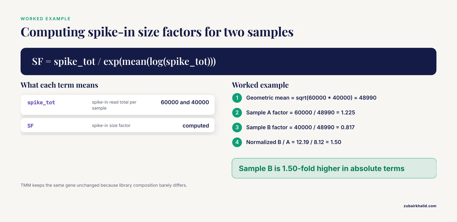
Put concrete numbers on the difference between relative and absolute normalization. Two libraries were sequenced to the same depth, but sample B contains about 1.5 times more RNA per unit of spike-in.
| Quantity | Sample A | Sample B |
|---|---|---|
| , - | , - | , - |
| Total reads | 10,000,000 | 10,000,000 |
| Spike-in reads | 60,000 | 40,000 |
| Endogenous reads | 9,940,000 | 9,960,000 |
Geometric mean spike total = sqrt(60000 * 40000) = 48990
Sample A size factor = 60000 / 48990 = 1.225
Sample B size factor = 40000 / 48990 = 0.817
Normalized endogenous A = 9940000 / 1.225 = 8.12 million
Normalized endogenous B = 9960000 / 0.817 = 12.19 million
Fold change, B versus A = 12.19 / 8.12 = 1.50
A gene with 1,000 raw counts in both samples stays essentially unchanged under TMM, because the endogenous library sizes and compositions are nearly identical. Under spike-in normalization the same gene is 1.5-fold higher in sample B, because B holds more RNA per spike-in molecule. Neither answer is wrong, they answer different questions, and the drug-treatment study above shows the absolute question is sometimes the one that matters.
Troubleshooting Spike-in Normalization
Most bioinformatics troubleshooting in this workflow reduces to one theme: the spike-ins were never measured, or they were measured badly. The table lists the failures seen most often, with exact messages where the software provides them.
| Message or symptom | Cause | Fix |
|---|---|---|
| , - | , - | , - |
Error: size factors should be positive from DESeq2 | All spike-in rows are zero, usually because ERCC is missing from the index or the grepl pattern does not match the row names | Rebuild the reference with ERCC included and confirm table(is_spike) reports 92 |
Warning ... NaNs produced from mean(log(spike_tot)), followed by nonsense factors | One sample has zero spike-in reads | Inspect that library, check the spike addition record, redesign the amount or drop the sample |
| featureCounts reports zero reads for every ERCC gene | ERCC absent from the GTF, or chromosome names differ between FASTA and GTF | Regenerate the combined annotation with identical names in both files |
| Salmon maps almost no spike-in reads | ERCC sequences missing from the transcriptome FASTA used to build the index | Rebuild the index from the combined FASTA |
negative values not allowed from calcNormFactors | TMM was run on non-integer or offset-corrected values | Run normalization on raw integer counts |
| Spike-in percentage varies several-fold across samples | Inconsistent pipetting, different dilutions, or different lots across batches | Re-add from one master dilution and record every volume in the sample sheet |
Silent failures deserve their own warning. A missing ERCC block in the annotation produces a perfectly ordinary looking count matrix with zero spike rows, and the workflow only breaks later, at the size factor step. The table(is_spike) check in Step 4 exists to catch that early, and it costs one line of R.
Common Mistakes and Limitations
- Adding the spike-ins at the wrong step for the question. Spike-ins in the lysis buffer track extraction, spike-ins added after mass loading track library preparation only, and per-cell addition in single-cell experiments enables absolute per-cell estimates. Mixing up the three designs produces numbers that look fine and mean something else.
- Loading equal RNA masses when the goal is absolute change. Mass loading mathematically removes total RNA differences before the spike-ins ever see them, so the design can only report relative results no matter how carefully the controls were added.
- Trusting raw ERCC size factors when the measurements are noisy. The direct evaluation by Risso and colleagues found ERCC controls not reliable enough for standard global-scaling or regression-based normalization, which is why RUVg exists [8]. If your observed-versus-expected plots wobble at low concentrations, move to RUV rather than forcing the factors.
- Reading spike-in fold changes as relative changes, or TMM fold changes as absolute ones. The two scales diverge exactly when global transcription shifts, as the worked calculation shows, and the drug-treatment study demonstrates how the absolute view can carry the biology [3].
- Forgetting the controls in the reference. This is the zero-rows failure from the troubleshooting table, and it is silent until Step 5.
- Letting spike-in amounts vary across batches. Different lots, dilutions, or volumes turn the reference into a batch confound, and no downstream method can recover the intended scale.
- Choosing a differential expression method from spike-in-only benchmarks. Such datasets contain technical variability only, and rankings of methods including edgeR, DESeq2, and limma-voom variants differ between spike-in and simulation benchmarks [9].
- Transferring plate-based spike-in practice to droplet data without thinking. ERCC-aware methods won on dilution-based single-cell data [5], but current droplet workflows often do better with endogenous methods such as Dino or scTransform [7]. Match the method to the platform and the question.
- Expecting spike-ins to remove gene-specific batch effects. They capture global scale, not per-gene artifacts. Unwanted variation that differs across genes needs factor-analysis approaches like RUV [8].
- Assuming the normalization choice only rescales fold changes. Normalization interacts with the test itself and with winsorization to shape false positive rates, and correspondence analyses of differential expression methods show the test choice matters as much as the scaling [11].
- Using relative normalization on small RNA-seq data with shifting populations. Common relative approaches can drive erroneous conclusions when the small RNA population itself fluctuates between tissues, which is why dedicated synthetic sRNA spike-in sets were developed [12].
Limitations. Spike-in normalization measures whatever the design makes it measure, so the absolute-versus-relative choice is a scientific decision, not a software setting. The assumptions behind any method, spike-in or endogenous, must be checked against the experiment rather than assumed [2]. Method performance also varies with the dataset, and tools such as NormSEQ evaluate candidate normalization methods on your own data using information gain to guide selection [13]. Individual datasets, especially those with unusual designs or strong batch structure, deserve review by an experienced analyst before the results feed a decision.
Practical Tips for Reliable Spike-in Normalization
- Run a pilot to place the spike-in fraction in a small, stable range with enough spike reads to keep the factor stable.
- Make one master dilution, aliquot it, freeze it, and use the same lot for the whole study.
- Randomize conditions across extraction batches and sequencing lanes so the reference is shared.
- Produce a one-page QC report per sample: spike-in percentage, observed-versus-expected correlation, and the size factor.
- Plot spike-in factors against TMM factors for every experiment, and investigate any sample far from the diagonal.
- Keep ERCC identifiers consistent across FASTA, GTF, tx2gene, and the analyte table from day one.
- For challenging designs, consult evaluations on difficult normalization scenarios before committing, since common methods have documented shortcomings there [14].
- Consider a validated endogenous reference such as mitochondrial mRNA as an alternative. A preprint reports it performed better than exogenous spike-ins and reduced batch effects, so validate it in your own system before adopting it [15].
Alternatives and Special Cases
Near-neighbor RNA as an internal standard. Yu and colleagues used chimpanzee RNA as a spike-in standard for human RNA-seq experiments. Human and chimpanzee transcripts carry single nucleotide variations at average intervals of about 210 base pairs, so chimpanzee RNA behaves like the human counterparts through the whole next-generation sequencing procedure, and reads are assigned to a species using those variants. The approach normalized as many as 10,119 transcripts read-by-read and made datasets degraded in process or prepared with different library methods comparable [16].
Small RNA-seq. Locati and colleagues built two synthetic sets: a size-range quality control (SRQC) set of 11 oligoribonucleotides from 10 to 70 nucleotides that tracks biases in size selection, and an external reference for data normalization (ERDN) set of 19 oligoribonucleotides that supported differential expression detection across a dynamic range of 2^18 [17]. Lutzmayer and colleagues developed sRNA spike-ins that enable absolute normalization across independent experiments and, combined with mRNA spike-ins, genome-wide estimates of sRNA to mRNA stoichiometry [12].
The same idea in ChIP-seq. The spike adjustment procedure adds a constant low amount of foreign-genome chromatin before immunoprecipitation, and that spike serves as an internal reference which improved replicate similarity and revealed uniform global occupancy changes that standard normalization missed [18].
Targeted panels. On TempO-Seq data, upper quartile normalization preserved simulated fold changes best, with specificity above 0.84 and sensitivity above 0.90 at most fold change levels [10].
Per-gene refinement. Two-stage methods that scale samples globally and then normalize per gene (Med-pgQ2 and UQ-pgQ2) achieved slightly higher AUC, specificity above 85 percent, detection power above 92 percent, and an actual false discovery rate under 0.06 on MAQC2 data with two replicates [19].
Downstream consequences. Normalization choice propagates further than the differential expression table. In condition-specific genome-scale metabolic modeling, data normalized by RLE, TMM, or GeTMM produced models with considerably low variability, while other choices changed model content [20].
Frequently Asked Questions
What is spike-in normalization in RNA-seq?
It is a normalization strategy that scales each sample by the reads mapped to synthetic RNA controls of known sequence and concentration, such as the 92 ERCC transcripts, added in a fixed amount to every sample. Dividing by a spike-in-derived size factor places samples on an absolute scale rather than a relative one.
When should I use spike-in normalization instead of TMM or DESeq2 normalization?
Use it when global transcription or total RNA per sample can genuinely change, when you need absolute per-cell quantities in single-cell experiments, or when the assumptions of relative methods are otherwise violated. Stay with TMM or DESeq2 factors when most genes are expected unchanged and total RNA is stable, because endogenous methods are less noisy.
How much ERCC spike-in should I add to each sample?
Add the same amount of the same mix to every sample, at a dilution chosen in a pilot so spike-ins are a small, stable fraction of reads with enough spike counts to estimate the factor reliably. Never vary the amount between samples, and record the lot and dilution in the sample sheet.
Why are all my ERCC spike-in counts zero?
Almost always because the ERCC sequences were never added to the alignment index or the annotation used for counting. Rebuild the reference with ERCC included, keep identifiers identical across files, and confirm with a quick row-count check before computing factors.
Can ERCC spike-ins remove batch effects?
Only global scaling differences between samples. Gene-specific batch artifacts need factor-based correction such as RUV, which uses the spike-ins as control features rather than as direct scaling factors.
Do spike-ins work in single-cell RNA-seq and droplet platforms like 10x?
They work well in plate-based, full-length protocols where they can be added per well, and ERCC-aware methods outperformed non-spike-in methods on dilution-based single-cell data. Droplet 10x data is commonly normalized with strong endogenous methods such as Dino or scTransform, so spike-ins are optional there unless absolute per-cell questions matter.
What can I use instead of ERCC spike-ins?
Options include near-neighbor RNA such as chimpanzee RNA for human samples, dedicated synthetic sets for small RNA-seq, mitochondrial mRNA as an endogenous reference after validation, and standard endogenous methods like TMM, RLE, or modern single-cell normalizers when relative assumptions hold.
Do spike-ins change my differential expression results?
Yes, whenever total RNA output differs between conditions. Genes moving with the global shift gain fold change under spike-in normalization while relative methods compress the signal toward zero, so gene rankings and the set of significant hits can change substantially.
Sources
- A scaling normalization method for differential expression analysis of RNA-seq data
- Selecting between-sample RNA-Seq normalization methods from the perspective of their assumptions
- Spike-in normalization for single-cell RNA-seq reveals dynamic global transcriptional activity mediating anticancer drug response
- Correction to ‘Spike-in normalization for single-cell RNA-seq reveals dynamic global transcriptional activity mediating anticancer drug response’
- Assessment of Single Cell RNA-Seq Normalization Methods
- Normalization Methods on Single-Cell RNA-seq Data: An Empirical Survey
- Single-cell RNA-seq data normalization: A benchmarking study
- Normalization of RNA-seq data using factor analysis of control genes or samples
- Benchmarking RNA-seq differential expression analysis methods using spike-in and simulation data
- Comparison of Normalization Methods for Analysis of TempO-Seq Targeted RNA Sequencing Data
- Response to "Neglecting normalization impact in semi-synthetic RNA-seq data simulation generates artificial false positives" and "Winsorization greatly reduces false positives by popular differential expression methods when analyzing human population samples"
- Novel small RNA spike-in oligonucleotides enable absolute normalization of small RNA-Seq data
- NORMSEQ: a tool for evaluation, selection and visualization of RNA-Seq normalization methods
- Evaluation of RNA-seq normalization methods using challenging datasets
- Mitochondrial mRNA is a stable and convenient reference for the normalization of RNA-seq data
- Normalization of human RNA-seq experiments using chimpanzee RNA as a spike-in standard
- Improving small RNA-seq by using a synthetic spike-in set for size-range quality control together with a set for data normalization
- Quantifying ChIP-seq data: a spiking method providing an internal reference for sample-to-sample normalization
- A comparison of per sample global scaling and per gene normalization methods for differential expression analysis of RNA-seq data
- A benchmark of RNA-seq data normalization methods for transcriptome mapping on human genome-scale metabolic networks