Scaling Single-Cell RNA-Seq Analysis in the Cloud
By Dr. Zubair Khalid, DVM, MS, PhD ·
By the end of this guide you will be able to move a single-cell RNA-seq project from a laptop to a cloud environment, run a reproducible preprocessing and clustering workflow on Amazon Web Services (AWS), keep the bill under control with spot instances and workflow caching, and validate that your scaled-out results match what a local run would produce. You will need an AWS account with permissions to create S3 buckets and Batch compute environments, Nextflow (version 23 or later) installed locally or in a container, Docker or Apptainer for containerized tools, roughly 20 GB of free disk for references and intermediates, and a small test dataset such as a 10x Genomics sample with a few thousand cells.
Why Single-Cell RNA-Seq Outgrows the Laptop
A single 10x Genomics lane can yield tens of thousands of cells. Multiplexed experiments, tissue atlases, and pooled CRISPR screens routinely push datasets past one million cells, and analysis demands grow faster than cell counts because clustering, neighborhood graphs, and differential expression all scale super-linearly with the number of cells. The ICARUS v3 web server was built specifically for this regime, and its developers demonstrate analysis of a 1.3 million cell dataset completed within the hour by using geometric cell sketching to subsample for dimensionality reduction and then project results back to the full dataset [1].
A laptop with 16 GB of RAM struggles once the count matrix alone reaches tens of gigabytes. An HPC cluster works, but most clusters are queue-constrained, and interactive exploration of a million-cell object is painful when you get 15 minutes of GPU time per session. Cloud computing removes both constraints. You provision exactly the memory and CPUs your step needs, you pay only while the step runs, and you can fan a 200-sample preprocessing job across hundreds of parallel tasks. This is the core promise of cloud bioinformatics, and it is the reason production platforms for genomics now run almost entirely on cloud infrastructure. The Celeste architecture supporting the All of Us Research Program processed workloads of up to 9,000 whole-genome samples per month using serverless technology and container orchestration within a single AWS Region, coordinating around 1.8 million jobs in a year of production [2]. The same architectural ideas apply directly to single-cell RNA-seq (scRNA-seq).
Scaling in the cloud is not only about speed. It changes what analyses become practical. You can re-run preprocessing from FASTQ files after a change in reference annotation, test three clustering resolutions in parallel, or sweep a whole cohort for batch effects overnight instead of negotiating cluster time. Cloud-based frameworks have demonstrated substantial efficiency gains over conventional local frameworks while maintaining or improving result quality, as benchmarked on the Human Cell Atlas Census of Immune Cells bone marrow dataset [3].
Core Vocabulary for Cloud Bioinformatics
Before running anything, you need five concepts firmly in place. Every step of the walkthrough below uses them.
Object storage. On AWS this is S3. Buckets hold FASTQ files, reference genomes, count matrices, and workflow outputs. Object storage is cheap, versioned, and readable from any compute node, which makes it the backbone of cloud pipelines. Compute never lives long, but data in S3 does.
Elastic compute. Virtual machines (EC2 instances) come in families sized for memory (R-family), compute (C-family), or accelerators (P- and G-family GPUs). Instead of choosing one machine, workflow engines request a fleet of them through a batch service. AWS Batch provisions instances, runs your jobs as containers, and tears everything down when the queue empties.
Spot instances. These are spare cloud capacity offered at steep discounts, with the caveat that AWS can reclaim the machine on short notice. Falco, an early cloud framework for scRNA-seq built on Apache Hadoop and Apache Spark, showed that using low-cost spot instances of Amazon Web Services reduces analysis cost by roughly 65 percent, while the same pipeline runs 2.6 to 145.4 times faster than on a highly optimized standalone computer [4]. Spot pricing is the single biggest cost lever in aws genomics work, provided your workflow tolerates interruptions.
Containers. A container bundles a tool with its exact dependencies so it runs identically on your laptop, an EC2 node, or a university cluster. The nf-core ecosystem, which hosts community-maintained pipelines for sequencing analysis, requires full containerization precisely because it guarantees reproducibility and scalability across diverse compute environments [8].
Workflow engines. Nextflow, WDL (with Cromwell), and CWL describe a pipeline as a graph of steps with declared inputs, outputs, and resource requests. The engine handles parallelization, retries, caching, and logging. Portable workflow definitions can be published to Dockstore and run on different platforms, an approach demonstrated by rMATS-cloud, which provides the same analysis as CWL, WDL, and Nextflow and was evaluated on the Cavatica, Terra, and Seqera platforms [5].
Three Architectures for Scaling Single-Cell RNA-Seq Analysis in the Cloud
There is no single right way to scale. Most projects fall into one of three patterns, and it is worth deciding explicitly which one fits your team before provisioning anything.
| Pattern | What you run | Best for | Main cost lever | Example |
|---|---|---|---|---|
| Managed pipeline platform | Prebuilt workflows submitted through a web interface | Wet-lab collaborators, standardized processing | Platform efficiency and shared resources | Cumulus, AnVIL |
| Workflow engine you operate | Nextflow, Cromwell, or cwlflex running on AWS Batch | Labs with informatics support and custom pipelines | Spot instances, task parallelism | nf-core/scrnaseq on Batch |
| Interactive web service | Browser-based analysis of preloaded or uploaded data | Exploration, million-cell visualization, no-code analysis | Sketching and subsampling algorithms | ICARUS v3 |
Cumulus is the reference example of the first pattern. It is a cloud-based framework for large-scale single-cell and single-nucleus RNA-seq that combines cloud computing with improvements in algorithm and implementation to achieve high scalability, low cost, user-friendliness, and integrated support for a comprehensive set of features including cell clustering and differential expression [3]. If your goal is to process a cohort to a standard deliverable with minimal infrastructure work, a managed platform is usually the correct answer.
The second pattern gives you full control. You own the workflow definition, the container versions, and the compute configuration. This is the pattern the step-by-step walkthrough below uses, because it teaches you every moving part and transfers directly to other pipelines.
The third pattern covers hosted analysis servers. ICARUS v3 is a massively scalable web server for scRNA-seq analysis of millions of cells, and its sketching approach means you can explore a million-cell dataset interactively without ever provisioning a cluster yourself [1]. The National Microbiome Data Collaborative took a similar layered approach for microbiome multi-omics with NMDC EDGE, whose architecture separates a web application layer, an orchestration layer, and an execution layer built on containers that accommodate both high-performance computing and cloud services [6]. The layered separation is a good design target for any team building its own internal platform.
Step-by-Step: A Scalable scRNA-Seq Workflow on AWS
This walkthrough preprocesses a batch of 10x Genomics samples through FASTQ alignment, count matrix generation, doublet detection, and initial clustering, then moves the merged object to scalable downstream analysis. The same logic applies to Azure or Google Cloud with services that map one-to-one.
Step 1. Prepare storage and references
Create a bucket with a naming convention that separates raw reads, references, and results. Enable versioning on the results prefix so that pipeline reruns never silently overwrite outputs.
aws s3 mb s3://scrnaseq-lab-2026
aws s3api put-bucket-versioning \
    -bucket scrnaseq-lab-2026 \
    -versioning-configuration Status=Enabled

aws s3 mb s3://scrnaseq-lab-2026
mkdir -p refs && cd refs
# Cell ranger reference (10x Genomics prebuilt human reference)
wget https://cf.10xgenomics.com/supp/cell-exp/refdata-gex-GRCh38-2024-A.tar.gz
tar -xzf refdata-gex-GRCh38-2024-A.tar.gz

aws s3 sync refdata-gex-GRCh38-2024-A s3://scrnaseq-lab-2026/refs/human-GRCh38-2024-A/
aws s3 sync ../fastq s3://scrnaseq-lab-2026/fastq/
Expected result of the last command looks like this:
upload: fastq/sample01_S1_L001_R1_001.fastq.gz to s3://scrnaseq-lab-2026/fastq/sample01_S1_L001_R1_001.fastq.gz
upload: fastq/sample01_S1_L001_R2_001.fastq.gz to s3://scrnaseq-lab-2026/fastq/sample01_S1_L001_R2_001.fastq.gz
Tips that save hours later. Store the reference once and point every job at it through a bucket path, never copy it into each sample directory. Keep sample sheets in CSV with columns for sample ID, FASTQ paths, and expected cell counts, because every workflow in this article consumes a sample sheet. Set lifecycle rules so raw FASTQs move to infrequent-access storage after 90 days, since you rarely re-read them but must not lose them.
Step 2. Configure the workflow engine
Nextflow is the most common engine for this pattern, and nf-core/scrnaseq is a community-maintained scRNA-seq workflow built to nf-core standards with full containerization [8]. Put all parameters in a config file rather than on the command line, which keeps runs reproducible and avoids long argument strings.
// nextflow.config
workDir = 's3://scrnaseq-lab-2026/work'

process {
  executor = 'awsbatch'
  withLabel: 'process_high' {
    cpus = 16
    memory = 64.GB
  }
}

aws {
  region = 'us-east-1'
  batch {
    maxParallelTransfers = 8
    fuseEnabled = true
  }
}

params {
  input = 's3://scrnaseq-lab-2026/samplesheet.csv'
  fasta = 's3://scrnaseq-lab-2026/refs/human-GRCh38-2024-A/fasta/genome.fa'
  gtfa  = 's3://scrnaseq-lab-2026/refs/human-GRCh38-2024-A/genes.gtf.gz'
  aligner = 'star'
  protocol = '10X'
}
Run it:
export AWS_DEFAULT_REGION=us-east-1
nextflow run nf-core/scrnaseq -r 3.2.0 \
    -profile batch \
    -w s3://scrnaseq-lab-2026/work \
    -with-report run_report.html \
    -resume
The -resume flag is your most important scaling tool. It hashes every task's inputs and skips any task whose inputs, container, and parameters are unchanged, so a rerun after fixing one sample costs minutes rather than hours. Combined with spot-aware retry directives, resume makes interrupted spot instances an inconvenience instead of a disaster.
Expected console output at startup:
Launching `nf-core/scrnaseq` [soggy_curie] DSL2 - revision: 3.2.0 [GRCh38]
Selected process profile: 'batch'
------------------------------
  [a1/b2] COUNTMATRICS (sample01): STARTED
  [c3/d4] COUNTMATRICS (sample02): STARTED
  ...
Step 3. Size the compute correctly
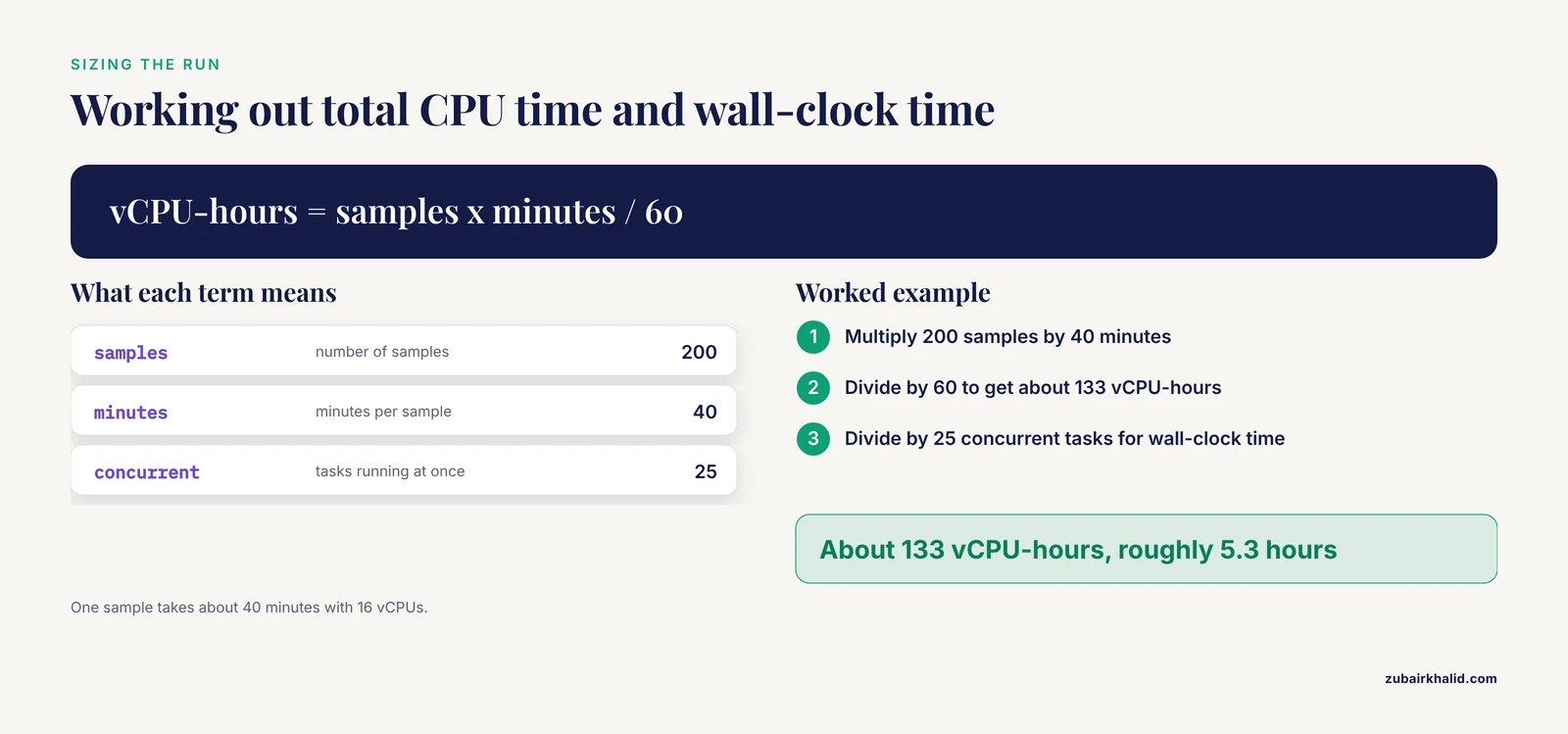
The most common scaling error is provisioning for the worst-case step and running the whole pipeline on that shape. Instead, assign resources per process label. A useful sizing exercise before launching: if you have 200 samples and empirically one sample takes about 40 minutes with 16 vCPUs, total CPU time is 200 times 40 divided by 60, or about 133 vCPU-hours. With 25 concurrent tasks the wall-clock time is roughly 5.3 hours. That arithmetic, not vendor marketing, should drive your Batch job queue limits.
A concise reference for common sizing decisions:
| Step | Typical bottleneck | Sensible shape | Parallelism |
|---|---|---|---|
| FASTQ alignment and counting (per sample) | CPU and RAM during genome index use | 16 vCPU, 64 GB | Per-sample, fully parallel |
| Ambient RNA and doublet correction (per sample) | RAM | 8 vCPU, 32 GB | Per-sample, fully parallel |
| Integration and clustering (merged object) | RAM, sometimes GPU | 96 vCPU, 768 GB, optional GPU | Single large task |
| Differential expression (per cluster) | CPU | 8 vCPU, 32 GB | Per-cluster, fully parallel |
Step 4. Control cost while it runs
Three habits keep an AWS genomics project affordable. First, use spot instances for every per-sample task and configure the workflow to retry automatically on spot reclamation, following the practice Falco demonstrated for scRNA-seq pipelines [4]. Second, cap concurrency with a Batch job queue maximum so a forgotten run cannot spawn 500 instances. Third, delete or expire the work directory aggressively. On S3-backed work directories, staged intermediates can quietly accumulate terabytes.
At the end of every session:
nextflow clean -f -before $(date -d "3 days ago" +%s)
aws s3 rm s3://scrnaseq-lab-2026/work/ -recursive \
    $(aws s3 ls s3://scrnaseq-lab-2026/work/ | awk '{print $2}')
In practice, verify with aws s3 ls and a billing console check that the Cost Explorer daily curve drops to near zero after the queue drains. A daily curve that stays flat means something is still running, and finding it a week later is the most expensive lesson in cloud bioinformatics.
Step 5. Verify the result is correct
Scaling introduces new failure modes, so validate against biology and against a small local run before trusting a million-cell output. For each sample, check mapping rate, median genes per cell, doublet fraction, and the ambient RNA profile. Then compare a 5,000-cell subset processed in the cloud against the same subset processed locally with the same container. Cell type proportions should agree within sampling noise. The benchmarking philosophy behind Cumulus, which maintained or improved quality of results while improving efficiency on the Human Cell Atlas bone marrow benchmark, is the standard to hold your own pipeline to [3].
A quick sanity check in Python on the merged output:
import scanpy as sc
adata = sc.read_h5ad("merged_annotated.h5ad")
print(adata.shape)                 # expect n_cells x ~30k genes
print(adata.obs["sample"].value_counts())
print(adata.obs["doublet"].mean()) # expect low single-digit percent
sc.tl.pca(adata, n_comps=30)
sc.pp.neighbors(adata, n_neighbors=15)
sc.tl.leiden(adata, resolution=1.0, key_added="leiden")
Expected output:
(1187432, 33538)
sample
s01    48213
s02    46905
...
doublet    0.021
Step 6. Scale downstream analysis with algorithms, not just hardware
Throwing vCPUs at clustering stops working somewhere between a few hundred thousand and a few million cells, because k-nearest-neighbor graph construction grows super-linearly. Two algorithmic strategies dominate. The first is sketching. ICARUS v3 uses geometric cell sketching to subsample cells for dimensionality reduction and clustering, then projects labels to the full dataset, and extends the representative subset to differential expression, co-expression networks, trajectory analysis, and cell-cell communication inference [1]. The second is feature reweighting. TF-IDF based clustering methods, adapted from text analysis, transform the count matrix so that genes restricted to small cell populations are upweighted, and empirical results show TF-IDF methods consistently outperform commonly used scRNA-seq clustering approaches on noisy, high-dimensional data [7]. TF-IDF is cheap to compute, which makes it attractive at scale:
import numpy as np
X = adata.raw.X                      # sparse counts
tf = np.log1p(X)
idf = np.log1p(adata.n_obs / (X > 0).sum(axis=0)).A1
adata.layers["tfidf"] = tf.multiply(idf)
Parallel statistical methods follow the same pattern. GLM-EIV, a method for single-cell CRISPR screen analysis that corrects attenuation bias in thresholded regression, was deployed across hundreds of processors on clouds such as Microsoft Azure to analyze two large-scale screen datasets [8]. The lesson generalizes: per-cell and per-cluster statistics parallelize embarrassingly well in the cloud, and the cloud is where they become tractable.
Step 7. Specialized analyses reusing the same infrastructure
The architecture you built is not scRNA-seq specific. Vulture, a cloud-enabled pipeline for detecting microbial reads in public scRNA-seq data, reuses the same pattern of fan-out compute over cloud object storage, and its benchmarking showed it was 66 to 88 percent faster than local tools and about 41 percent faster than the state-of-the-art cloud-based tool Cumulus, with cloud costs reduced from 70 dollars to 12 dollars per analysis [9]. If your scRNA-seq study might carry host-microbe signals, the same bucket-and-batch skeleton supports that pipeline with no new infrastructure. Conversely, if your analysis portfolio extends to alternative splicing or epigenomics, portable workflow definitions such as rMATS-cloud's CWL, WDL, and Nextflow packages on Dockstore can be dropped into the same compute environment [5], and platform efforts like EAP for large-scale ChIP and ATAC-seq demonstrate the same principle of configuration-free scalable analysis in the cloud [10].
Using AnVIL When You Prefer R
Not every team wants to operate Batch queues. The AnVIL ecosystem provides cloud-based genomics analysis with data and workflows already co-located, and the AnVILWorkflow R package lets you browse, launch, and retrieve results from hosted workflows directly from an R environment, handling environment setup, input formatting, submission, and result retrieval through intuitive functions [11]. For a lab whose analysts live in R, starting from AnVILWorkflow is often faster than assembling your own stack, and it retains the scalability benefits without direct infrastructure management. The tradeoff is less flexibility in custom pipeline steps.
Common Mistakes and Limitations
These are the errors that show up repeatedly when labs first scale single-cell RNA-seq analysis in the cloud, with concrete fixes.
- No checkpointing before spot use. Spot reclamation is routine, not exceptional. Configure Nextflow retry directives with incremental backoff and always run with
-resume. A workflow that cannot resume turns the 65 percent spot savings reported for Falco [4] into 65 percent wasted spending.
- Forgetting resources after a run. An idle EC2 instance or an unattached EBS volume bills forever. Adopt a daily teardown check: the Batch queue is empty, no instances are running, and Cost Explorer shows the expected decay to near zero.
- Treating the work directory as permanent. Work directories hold intermediate files that the workflow can regenerate. Leaving them in standard storage is one of the largest hidden costs in cloud genomics. Expire them with lifecycle rules or delete them after each successful run.
- Downscaling QC to save time. Skipping per-sample doublet and ambient RNA checks to cut compute time produces a merged object where one bad sample distorts every downstream cluster. Run QC at full parallelism, since it is the cheapest stage of the pipeline.
- Applying PCA to raw counts. Some pipelines carried over from bulk RNA-seq normalize once and run PCA on everything. On sparse single-cell data, use library-size normalization with log transformation for standard analyses, or TF-IDF style transformations for clustering, where they have demonstrated consistent performance advantages [7].
- Ignoring privacy obligations. Single-cell transcriptomics data can carry patient re-identification risk, and leaked genomic data is effectively unrecoverable because retraction is impossible. Privacy-preserving frameworks for transcriptomics clustering combine map-reduce parallelization with secure enclaves such as Intel SGX to protect data during processing [12]. At minimum, encrypt buckets at rest, restrict bucket policies to your pipeline roles, and never stage human data onto personal machines.
- Assuming one instance size fits all steps. A 768 GB integration node idles 90 percent of the time during per-sample counting. Per-process resource labels, as shown in the config above, typically cut total compute spend substantially compared to a uniform shape.
- Not validating against a small local run. Cloud scaling amplifies whatever your pipeline does, including its bugs. The comparison subset approach in Step 5 is non-negotiable for publication-grade results.
Two honest limitations deserve a place here. First, managed platforms trade flexibility for convenience, so if your protocol needs a nonstandard quantification method, confirm the platform supports it before committing a cohort. Second, cloud bills fluctuate with experiment design in ways local hardware does not, and a project with no budget monitoring will find that out in the invoice rather than the dashboard. Individual project decisions about platforms, data governance, and cost ceilings need review by whoever owns informatics and compliance in your organization.
Performance Targets You Can Expect
Published benchmarks give you a reasonable envelope. Falco demonstrated 2.6 to 145.4 times speedup over a highly optimized standalone computer depending on dataset and pipeline, with roughly 65 percent cost reduction from spot instances [4]. Cumulus benchmarked on the Human Cell Atlas Census of Immune Cells bone marrow dataset and substantially improved efficiency over conventional frameworks while maintaining or improving result quality [3]. ICARUS v3 completed analysis of 1.3 million cells within the hour using sketching rather than brute-force scaling [1]. Vulture reported 66 to 88 percent speedups over local microbial-calling tools and reduced per-analysis cost from 70 dollars to 12 dollars on cloud systems [9]. Treat these as directional, since results depend on data, instance pricing at the time, and pipeline configuration, but they establish that cloud scaling of scRNA-seq is a solved engineering problem with published evidence.
Frequently Asked Questions
How large a dataset can cloud-based scRNA-seq pipelines handle?
Very large ones. Published frameworks have processed million-cell datasets, with ICARUS v3 demonstrating analysis of 1.3 million cells within the hour [1], and production cloud infrastructures in genomics routinely handle fluctuating workloads of thousands of samples per month [2].
Do I need to be a cloud engineer to scale single-cell RNA-seq analysis?
No, if you choose the right pattern. Managed platforms like Cumulus are designed for user-friendliness at scale [3], and R packages like AnVILWorkflow handle environment setup, submission, and result retrieval for you [11]. You do need engineering help if you want a custom workflow on raw Batch infrastructure.
What exactly is a spot instance and should I use one?
A spot instance is spare cloud capacity offered at a discount that the provider can reclaim on short notice. Yes, use them for parallelizable steps, since Falco demonstrated roughly 65 percent cost reduction using AWS spot instances for scRNA-seq processing [4], but always pair them with a resumable workflow and automatic retries.
Can I run everything from R without touching the command line?
Mostly. AnVILWorkflow lets you execute hosted cloud workflows from an R environment, including browsing available workflows and retrieving results [11]. Interactive cloud notebooks also run R with Bioconductor single-cell packages. Raw FASTQ preprocessing still benefits from a workflow engine underneath.
How do I keep patient data secure in the cloud?
Encrypt buckets at rest and in transit, scope access to dedicated pipeline roles, and prefer regions and services that meet your compliance obligations. For workloads with strict privacy needs, specialized frameworks combine parallel clustering with hardware enclaves such as Intel SGX to protect data during processing [12], reflecting the reality that leaked genomic data cannot be retracted.
Which workflow engine should I choose, Nextflow, WDL, or CWL?
Choose the one your community already uses. Nextflow dominates the nf-core ecosystem and is the default in this guide, while portable workflows published in all three languages, such as rMATS-cloud's Dockstore packages, show that the same analysis can be expressed in CWL, WDL, or Nextflow and run across multiple platforms [5].
When should I stay on a laptop or a local HPC instead of the cloud?
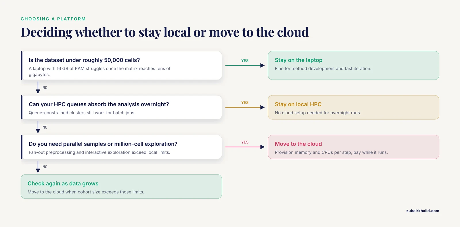
Stay local for datasets under roughly 50,000 cells, for method development where iteration speed on a familiar machine matters more than throughput, and for analyses your HPC queues can absorb overnight. Move to the cloud when cohort size, parallel sample processing, or interactive million-cell exploration exceeds those limits.
How do I make sure my scaled cloud run matches a local run?
Run the same container on the same 5,000-cell subset both ways and compare QC metrics, cell type proportions, and clustering assignments before committing the full cohort. Published cloud frameworks established this benchmarking standard, maintaining or improving result quality while improving efficiency at scale [3].
Sources
- ICARUS v3, a massively scalable web server for single-cell RNA-seq analysis of millions of cells.
- Celeste: A cloud-based genomics infrastructure with variant-calling pipeline suited for population-scale sequencing projects.
- Cumulus provides cloud-based data analysis for large-scale single-cell and single-nucleus RNA-seq.
- Falco: a quick and flexible single-cell RNA-seq processing framework on the cloud.
- rMATS-cloud: Large-scale Alternative Splicing Analysis in the Cloud.
- Standardized and accessible multi-omics bioinformatics workflows through the NMDC EDGE resource.
- Single cell RNA-seq data clustering using TF-IDF based methods.
- Exponential family measurement error models for single-cell CRISPR screens.
- Vulture: cloud-enabled scalable mining of microbial reads in public scRNA-seq data.
- EAP: A versatile cloud-based platform for efficient quantitative analysis of large-scale ChIP/ATAC-seq datasets.
- AnVILWorkflow: A runnable workflow package for Cloud-implemented bioinformatics analysis pipelines.
- PPPCT: Privacy-Preserving framework for Parallel Clustering Transcriptomics data.