RNA-Seq Quality Control with FastQC and MultiQC
By Dr. Zubair Khalid, DVM, MS, PhD ·

By the end of this article you will be able to run FastQC on an entire directory of RNA-seq FASTQ files, interpret every module in its report, trim adapters and low-quality bases with Cutadapt or fastp, and pull all of your samples into a single MultiQC report you can actually compare. These two tools open almost every published RNA-seq workflow. One representative example checks raw reads with FastQC and MultiQC, trims adapters with Cutalign, aligns with STAR, and quantifies transcripts with Salmon before differential expression testing [1]. Another recent study on intramuscular fat in cattle begins its methods the same way, with FastQC quality control followed by HISAT2 alignment and DESeq2 testing [2].
To follow along you need:
- A Linux, macOS, or Windows (WSL2) machine with at least 8 GB of RAM
- Conda or Miniforge installed, or permission to install software with your system package manager
- A directory of paired-end FASTQ files, ideally with meaningful sample names such as
SRR12345678_R1.fastq.gz - About an hour for the first pass on a small project
Whether you are working through a bioinformatics course or trying to learn bioinformatics on real sequencing data, this QC stage is the single best place to start, because every later conclusion depends on it.
Why Quality Control Comes First
RNA-seq turns RNA into numbers, and every number downstream inherits the condition of the reads it came from. A comprehensive treatment of RNA-seq analysis describes quality control as the step that lays the groundwork for everything that follows, from preprocessing to alignment to differential expression [3]. The reverse is also true. The SARTools pipeline documentation makes the point bluntly: quality control steps are recommended but not mandatory, and failing to check the characteristics of a dataset can lead to spurious results [4].
The stakes are not theoretical. In a systematic evaluation of 90 RNA-seq pipelines across rat, zebrafish, and mouse datasets with weak biological signals, the authors concluded that pipeline selection, starting from quality control, directly influences both analysis efficiency and the biological insights a study can deliver [5]. Two analysts given the same FASTQ files can reach different answers depending on how carefully they handled this stage.
Quality control also starts before sequencing in a practical sense. Ribosomal RNA makes up 80 to 90 percent of total cellular RNA, so inefficient rRNA depletion or poor poly(A) enrichment quietly floods a library with uninformative reads. A recent pre-sequencing assay showed that an 18S rRNA qPCR measurement correlates strongly with post-sequencing rRNA rates across thousands of libraries, which means some QC thinking should happen at the bench, before the flow cell is ever loaded [6]. If you receive data from a collaborator, rRNA fraction is one of the first things to look for in the raw-read report.
How FastQC and MultiQC Fit Into an RNA-Seq Workflow
A typical bulk RNA-seq workflow looks like this:
- Demultiplex the flow cell into per-sample FASTQ files (usually done by the sequencing facility).
- Run raw-read quality control with FastQC.
- Aggregate the per-sample reports with MultiQC and decide whether trimming is needed.
- Trim adapters and low-quality bases with a tool such as Cutadapt or fastp.
- Re-run FastQC on the trimmed reads and compare reports in MultiQC.
- Align or pseudoalign, quantify, normalize, and test for differential expression.
Published studies follow this shape closely. The influenza dataset paper cited above runs FastQC and MultiQC, trims with Cutadapt, filters reads with STAR, quantifies with Salmon, and calls differentially expressed genes with DESeq2 at an FDR-adjusted p-value below 0.001 and an absolute log2 fold change above 1 [1]. The cattle study uses FastQC before HISAT2 alignment and applies DESeq2 thresholds of p < 0.05 and |log2FC| > 0.5 [2]. Workflow engines such as 3t-seq, built on Snakemake, automate the same sequence of steps, performing quality control, genome mapping, gene expression quantification, and statistical testing directly from raw sequencing data with an accessible report at the end [7]. A plant-science pre-processing framework built for Arabidopsis thaliana Illumina data likewise treats rigorous quality control as the entry point to alignment, quantification, and normalization [8].
FastQC answers one question: what does this particular FASTQ file look like? MultiQC answers a different question: how do all of my files compare with each other? You need both, because a single sample can look acceptable in isolation and still stand out as an outlier when lined up against its cohort.
Installing FastQC and MultiQC
The cleanest route for most people is the Bioconda channel, which packages both tools plus the trimmers used later in this guide.
conda create -n rnaseq-qc -c conda-forge -c bioconda \
  fastqc multiqc cutadapt fastp

conda activate rnaseq-qc
Verify the installation:
fastqc --version
multiqc --version
cutadapt --version
fastp --version
If you cannot use conda, FastQC ships as a platform-independent package that runs under a Java installation, and MultiQC installs through pip (pip install multiqc). Cutadapt also installs through pip. FastQC's official documentation at the Babraham Bioinformatics site and MultiQC's documentation at multiqc.info cover both routes in detail.
A note on versions: FastQC's last major release predates many current sequencers, but the module logic remains the standard reference point. MultiQC, by contrast, is under active development and its parsers are updated regularly, so keep MultiQC reasonably current with conda update multiqc.
A Step-by-Step RNA-Seq Quality Control Workflow
The commands below assume this directory layout, which keeps raw data, QC output, and trimmed data separated:
project/
  reads/            raw FASTQ files
  trimmed/          trimmed FASTQ files
  qc/
    fastqc_raw/
    fastqc_trim/
    fastp/
    multiqc_raw/
    multiqc_compare/
Step 1: Inspect the raw FASTQ files
Before running anything, count your files and confirm read pairing. Every sample should have exactly two files, an R1 and an R2, with matching prefixes.
ls reads/ | wc -l
gunzip -c reads/Sample1_R1.fastq.gz | head -n 8
A FASTQ record is four lines: a header beginning with @, the sequence, a separator line beginning with +, and a base-quality string of the same length as the sequence. Check three things in the head output: the read name suffix (such as /1 or a trailing 1 in the header) confirms read number, the sequence length is consistent with what the facility promised, and the file decompresses without errors. A truncated FASTQ file, which happens when a download is interrupted, will fail later steps in confusing ways, so catching it now costs seconds instead of hours.
Step 2: Run FastQC on every file
mkdir -p qc/fastqc_raw

for f in reads/*.fastq.gz
do
  fastqc -o qc/fastqc_raw -t 8 "$f"
done
Two parameters matter here:
-osets the output directory. Without it, FastQC writes reports into the current directory.-tsets the number of threads. Each file gets its own thread, so-t 8processes eight files in parallel. This is the main speed lever, and it does not change results.
In the terminal you should see progress lines like this:
Started analysis of Sample1_R1.fastq.gz
Approx 5% complete for Sample1_R1.fastq.gz
Approx 10% complete for Sample1_R1.fastq.gz
Analysis complete for Sample1_R1.fastq.gz
FastQC writes two files per sample: a self-contained HTML report (Sample1_R1_fastqc.html) and a compressed archive (Sample1_R1_fastqc.zip). The HTML opens in any browser and works offline, which makes it easy to attach to a lab notebook or a project report. The zip contains the underlying data, including the fastqc_data.txt file that MultiQC parses later.
To unpack everything at once for command-line inspection:
for z in qc/fastqc_raw/*.zip
do
  unzip -o "$z" -d qc/fastqc_raw/
done
Step 3: Aggregate the reports with MultiQC
multiqc -o qc/multiqc_raw -n raw_fastqc qc/fastqc_raw-osets the output directory.-nnames the report. Naming raw and trimmed reports differently keeps them distinct when you compare them later.
Expected terminal output looks roughly like this:
  multiqc : This is MultiQC v1.x
  multiqc : Searching given paths: qc/fastqc_raw
  multiqc : bioinformatics : Found 12 reports for 'fastqc'
  multiqc : Compressing plot data
  multiqc : Report written to: qc/multiqc_raw/raw_fastqc.html
Open raw_fastqc.html in a browser. The header line, "multiqc: Found 12 reports for 'fastqc'" in this example, is your first correctness check. If you expected 24 files (12 samples, two reads each) and MultiQC found 12, something went wrong, usually a pattern-matching issue with file names.
The first table in a MultiQC report, General Statistics, gives you one row per file. An illustrative example of what a healthy paired-end lane might look like:
| Sample | M Reads | Length | % Dup | % GC |
|---|---|---|---|---|
| Sample1_R1 | 41.2 M | 150 | 12.5 | 51 |
| Sample1_R2 | 41.2 M | 150 | 12.5 | 51 |
| Sample2_R1 | 39.8 M | 150 | 10.9 | 50 |
| Sample2_R2 | 39.8 M | 150 | 10.9 | 50 |
Scan this table top to bottom before anything else. Read counts that differ wildly between samples, GC contents that spread across a range, or one sample with a duplication percentage far above the rest are all cohort-level signals that no single-sample report reveals.
Step 4: Interpret each FastQC module
Open any single-sample FastQC report and you will see roughly a dozen modules, each stamped with a traffic-light status: green for a normal result, orange for a warning, red for a failure. The most common beginner mistake in RNA-seq quality control is treating those stamps as verdicts. They are calibrated for generic sequencing, and several modules flag RNA-seq libraries in ways that are expected. The table below summarizes the modules that matter most and how to read them for this data type.
| FastQC module | What it measures | How to interpret it for RNA-seq |
|---|---|---|
| Basic Statistics | Read count, length, %GC | Confirm expected read count and length. Total RNA-seq libraries often show GC contents shifted by rRNA fraction, so compare across samples rather than to an absolute number. |
| Per base sequence quality | Phred score distribution at each cycle | Illumina runs decline toward the 3' end. Cycles dipping from Q30 toward Q20 near the tail are normal. Concern rises when median quality collapses early. |
| Per tile sequence quality | Quality by flow-cell tile | A warning here can indicate a physical flow-cell issue or a dirty run. It matters most when only part of the lane is affected. |
| Per sequence quality scores | Fraction of reads with low mean quality | A small low-quality tail is normal and handled by trimming. A large peak of poor reads suggests a systematic problem. |
| Per base sequence content | Base composition per cycle | Almost always flags random-primed RNA-seq libraries in the first 10 or so cycles because transcript sequences bias the first cycles. This is expected, not a defect. |
| Per sequence GC content | Distribution of GC per read | Compare the shape across samples. A shifted or bimodal distribution can indicate contamination or a changed library protocol. |
| Per base N content | Fraction of ambiguous bases | Should be near zero throughout. Rising N content late in the read is common and mostly cosmetic after trimming. |
| Sequence Length Distribution | Read length spread | Sharp and uniform for most modern runs. A smear of short fragments means heavy fragmentation or aggressive trimming already happened. |
| Sequence Duplication Levels | Fraction of duplicate reads | RNA-seq is naturally duplicate-rich because abundant transcripts are sequenced many times. High duplication matters more when library complexity, not expression, is the constraint. |
| Overrepresented sequences | Individual sequences appearing too often | In RNA-seq these are frequently genuine highly expressed transcripts, rRNA fragments, or adapters. Blast or align a handful of them before deleting anything. |
| Adapter Content | Adapter accumulation by cycle | The module that most directly drives a trimming decision. Rising adapter curves in the final cycles indicate inserts shorter than the read length. |
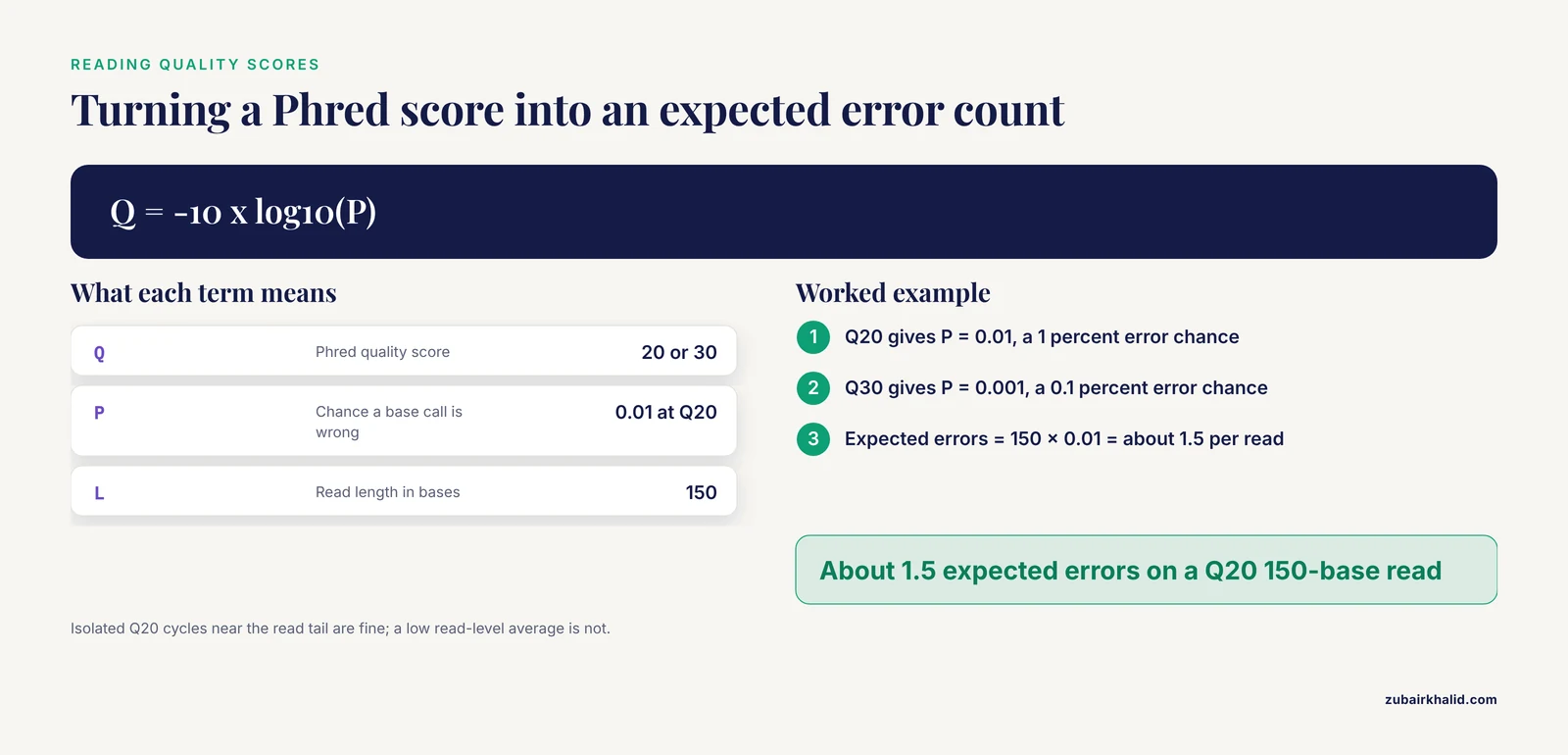
Two worked numbers help anchor the quality modules. The Phred score encodes the probability that a base call is wrong, with Q equal to minus 10 times the base-10 logarithm of that probability. Q30 therefore corresponds to a 1-in-1,000 error rate. On a 150-base read called entirely at Q20, the expected number of errors per read is 150 multiplied by 0.01, or about 1.5 errors, which is why read-level averages below Q20 deserve a closer look while isolated Q20 cycles near the end of a read do not.
The per-base sequence content module deserves its own explanation because it generates more false alarms than any other module. FastQC expects roughly equal proportions of A, C, G, and T at every cycle, which is true for shotgun genomic DNA. RNA-seq libraries are built with random priming, and the first several cycles reflect the biased composition of transcript fragments, so the module lights up orange or red on perfectly healthy libraries. Learn the shape of your own platform's early-cycle bias and treat deviations from your own baseline, rather than from FastQC's generic expectation, as the real signal.
Step 5: Trim adapters and low-quality bases
Two widely used tools cover this step. Cutadapt removes adapter sequences with precise, documented algorithms. fastp performs adapter trimming, quality filtering, and report generation in a single fast pass. The influenza dataset workflow cited earlier used Cutadapt for adapter and quality trimming between FastQC and STAR [1], and Cutadapt remains the reference choice when you need exact control over what is removed.
A standard paired-end Cutadapt invocation for Illumina libraries looks like this:
mkdir -p trimmed

cutadapt \
  -a AGATCGGAAGAGC \
  -A AGATCGGAAGAGC \
  -m 25 \
  -o trimmed/Sample1_R1.trim.fastq.gz \
  -p trimmed/Sample1_R2.trim.fastq.gz \
  reads/Sample1_R1.fastq.gz reads/Sample1_R2.fastq.gz
The parameters that matter:
-ais the 3' adapter expected on read 1, and-Ais the same for read 2.AGATCGGAAGAGCis the core of the standard Illumina adapter, and the TruSeq and similar families share this prefix. Confirm the exact sequence with your library kit documentation, because the correct adapter is a property of the kit, not a universal constant.-m 25discards read pairs where either partner falls below 25 bases. Keeping ultra-short fragments hurts alignment more than losing them does.- The input order is R1 then R2, and Cutadapt keeps pairs synchronized.
Cutadapt prints a summary to standard output, including the number of pairs processed, pairs written, and bases removed. Save that summary to a file so MultiQC can collect it:
cutadapt \
  -a AGATCGGAAGAGC \
  -A AGATCGGAAGAGC \
  -m 25 \
  -o trimmed/Sample1_R1.trim.fastq.gz \
  -p trimmed/Sample1_R2.trim.fastq.gz \
  reads/Sample1_R1.fastq.gz reads/Sample1_R2.fastq.gz \
  > qc/fastp/Sample1.cutadapt.log 2>&1
If you prefer an all-in-one tool, fastp trims adapters for paired-end data automatically through overlap analysis and writes an HTML report and a JSON file:
fastp \
  -i reads/Sample1_R1.fastq.gz \
  -I reads/Sample1_R2.fastq.gz \
  -o trimmed/Sample1_R1.trim.fastq.gz \
  -O trimmed/Sample1_R2.trim.fastq.gz \
  -h qc/fastp/Sample1.fastp.html \
  -j qc/fastp/Sample1.fastp.json \
  -w 8
Here -h and -j name the report files and -w sets threads. fastp's JSON output is one of the formats MultiQC parses directly, which is a major convenience for large projects.
For a batch of samples, wrap the call in a loop:
for r1 in reads/*_R1.fastq.gz
do
  base=$(basename "$r1" _R1.fastq.gz)
  fastp \
    -i "reads/${base}_R1.fastq.gz" \
    -I "reads/${base}_R2.fastq.gz" \
    -o "trimmed/${base}_R1.trim.fastq.gz" \
    -O "trimmed/${base}_R2.trim.fastq.gz" \
    -h "qc/fastp/${base}.fastp.html" \
    -j "qc/fastp/${base}.fastp.json" \
    -w 8
done
Step 6: Re-run FastQC and compare with MultiQC
fastqc -o qc/fastqc_trim -t 8 trimmed/*.fastq.gz

multiqc -o qc/multiqc_compare -n raw_vs_trim \
  qc/fastqc_raw qc/fastqc_trim qc/fastp
The comparison report places raw and trimmed samples in the same plots, and the General Statistics table now shows before-and-after read counts side by side. Check three things:
- Adapter content curves in the trimmed reports should flatten to near zero across the whole read.
- Per-base quality profiles should show the low-quality tail removed, with the median line staying near Q30 through most of the read.
- Read survival should be high. Poly(A)-selected libraries with heavy adapter content lose more, but a sample that lost a large fraction of its reads relative to its neighbors is a red flag worth investigating before alignment.
That comparison report is the artifact you archive. When a reviewer or collaborator asks how you judged data quality, the raw-versus-trimmed MultiQC report is the answer.
What Counts as Normal for RNA-Seq Data
RNA-seq libraries violate several generic FastQC expectations for reasons rooted in biology and library preparation, and knowing which warnings to accept separates confident QC from constant re-trimming.
Expect non-uniform per-base sequence content in the first cycles from random priming. Expect per-sequence GC content that reflects your transcriptome, with total RNA libraries pulled toward the GC content of rRNA when depletion is imperfect. Expect overrepresented sequences that align to abundant transcripts rather than to contamination. Expect moderate duplication, because a handful of highly expressed genes legitimately occupy a large share of the library.
What you should not accept: quality scores that collapse in the first half of the read, N content climbing above a few percent early in the read, adapter curves that rise steeply from mid-read rather than only at the tail, a GC distribution shape that differs between samples processed identically, or one sample with read counts far outside the cohort range. Each of those points to a concrete problem, from a failed rRNA depletion to a sample swap.
The Arabidopsis pre-processing study makes a related methodological point: optimal pre-processing parameters, including QC decisions, must be tuned to the organism and protocol at hand, and the authors built their framework specifically around those Illumina-specific considerations [8]. The practical translation is that your best reference population is your own experiment, run through MultiQC as a cohort.
One pre-sequencing control deserves mention because it prevents downstream surprises. Because rRNA dominates total cellular RNA, an inefficient depletion shows up as wasted sequencing depth. The 18S rRNA qPCR assay described across 1,748 total RNA-seq and 445 poly(A)+ libraries predicted post-sequencing rRNA rates before sequencing, which lets a facility re-prepare a failing library rather than sequence it and discover the problem in the FastQC report [6]. If you control the bench side, use it. If you only see the data afterward, rRNA fraction is visible in the overrepresented sequences module and in post-alignment metrics.
Practical Tips for Faster, Cleaner RNA-Seq Quality Control
These tips come from the parts of QC that cost the most time when done badly.
Run MultiQC on everything, always. MultiQC parses reports from dozens of tools, including FastQC, Cutadapt, fastp, and alignment and quantification software, into one HTML file. Even in a pipeline like 3t-seq that already produces an accessible report from raw data through differential testing, the underlying aggregation principle is the same: one place to see every sample at once [7].
Name samples before you run FastQC. MultiQC builds its tables from file names. Renaming sample1_R1.fastq.gz to liver_day0_rep1_R1.fastq.gz before QC means every downstream report, including the MultiQC General Statistics table, carries biological context for free.
Keep raw reports and trimmed reports in separate directories. When MultiQC is pointed at both directories in one call, it labels raw and trimmed data separately in the same plots, which is exactly the comparison you want. Mixing them in one directory scrambles that.
Snapshot your tool versions. Write fastqc, version, multiqc, version, and cutadapt, version into a versions.txt in the project directory. MultiQC can also record tool versions in its report. Reproducibility at QC costs one command.
Trust the cohort, not the stamps. The orange and red badges are heuristics written for generic sequencing. The multi-sample view in MultiQC, where you can see whether one sample deviates from twelve identical siblings, is a more reliable judge than any single badge.
For point-and-click workflows, use a wrapper. If command lines are a barrier, tools such as SEQUIN provide a web-based interface that includes quality control, gene set enrichment, visualization, and differential expression analysis for RNA-seq data from model organisms, tissues, and single cells [9]. Wrappers are fine for exploration, but keep the underlying command-line QC in your records for publication.
Automate the whole sequence when the project grows. Once a project exceeds a couple dozen samples, wrapping FastQC, MultiQC, and trimming in a workflow engine pays for itself. 3t-seq demonstrates the pattern, running quality control through statistical testing from raw data with configuration-managed dependencies [7], and the general finding that pipeline choice measurably affects results argues for locking your pipeline down in code rather than retyping it [5].
Common Mistakes and Limitations
These are the errors that most often produce wrong conclusions or wasted sequencing budget.
Treating every red FastQC flag as a data failure. The per-base sequence content module flags nearly all random-primed RNA-seq libraries in early cycles. Overrepresented sequences are often genuine transcripts. Blanket re-trimming to appease the badges wastes reads and changes nothing.
Trimming without evidence. If the adapter content module is flat across all cycles, adapter trimming removes nothing and only risks over-trimming legitimate bases. Trim when the report shows adapters or a degraded quality tail, and trim consistently across all samples in an experiment so that bias is uniform rather than sample-specific.
Comparing samples processed with different trimming settings. If one sample was trimmed at a minimum length of 25 and another at 50, downstream read counts reflect your choices as much as the biology. Apply one pipeline to one experiment.
Reading duplication as contamination. RNA-seq duplication largely reflects transcript abundance. High duplication in a small, deeply sequenced library is normal. Duplication only becomes alarming when it is inconsistent with library complexity expectations for the protocol, or when it appears suddenly in one sample of a matched cohort.
Ignoring pair synchronization. If you trim R1 and R2 in separate Cutadapt calls with different settings, pairs desynchronize and every paired-end aligner downstream will complain or silently misbehave. Always trim both mates in one call, as the Step 5 command does.
Skipping QC on a trusted facility's data. Published pipelines that begin with FastQC and MultiQC do so because even core-generated data varies with library prep batches and flow cells [1]. QC is cheap, roughly minutes per sample.
Forgetting that quality control has a single-cell edition. The FastQC modules discussed here operate on the FASTQ level and apply to any short-read data. Single-cell RNA-seq adds a second QC layer at the cell level, where the goal is identifying barcodes containing intact cells and flagging damaged ones. Dedicated single-cell methods are required because bulk pipelines cannot simply be recycled [10], and recent tools address exactly this, including data-adaptive barcode filtering that flags dead cells in single-cell and single-nucleus data [11], guided R packages that integrate pre-processing and QC parameter selection [12], unsupervised ensemble classifiers for cell quality [13], and consensus guidelines covering raw data processing and QC for biomedical and clinical applications [14]. The points above about cohort thinking, version recording, and consistent settings still apply in full.
Believing QC guarantees correct biology. Clean reads do not rescue a weak design. The 90-pipeline evaluation found that even with QC in place, pipeline choices shape whether weak biological signals survive analysis, and the authors ranked pipelines by agreement with qRT-PCR and by classifier performance rather than by QC metrics alone [5]. Tools such as SARTools embed diagnostic plots throughout normalization and testing because QC has to continue past the FASTQ stage, checking model assumptions before trusting a differential expression result [4]. Published differential expression studies routinely report PCA separating condition groups as an early sanity check that QC carried through the pipeline [15].
One boundary note. Individual sequencing runs and sample conditions vary, and any decision that affects a real study, especially around resubmitting or re-preparing a library, deserves a conversation with the sequencing facility or an experienced analyst rather than a fixed rule from a guide like this one.
Frequently Asked Questions
Do I always need to trim my RNA-seq reads before alignment?
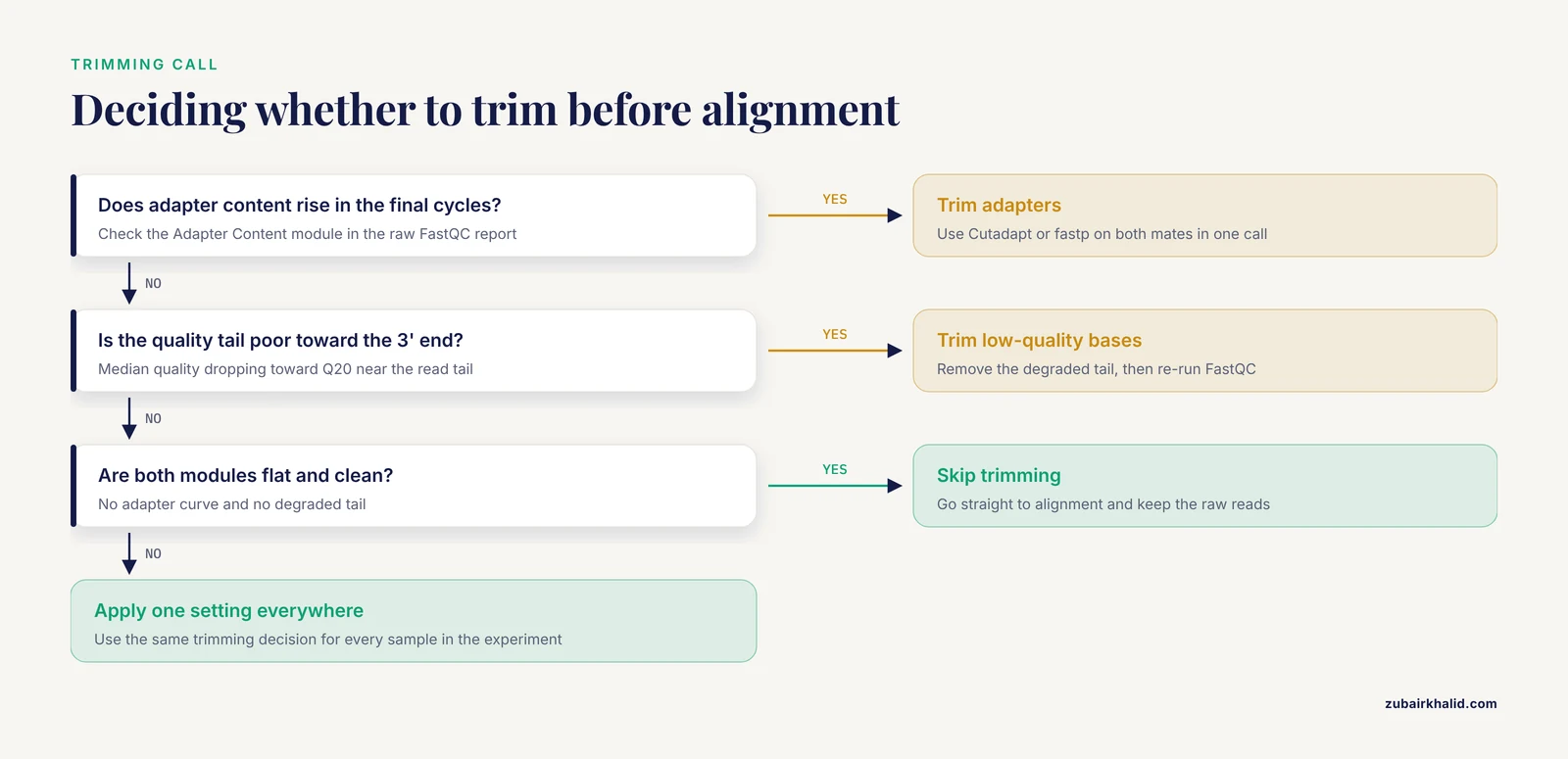
No. Trim when the FastQC adapter content module shows adapter accumulation or when the quality tail is poor, and skip it when neither appears. What matters is applying the same decision to every sample in the experiment.
Why does FastQC flag per-base sequence content as a failure on healthy RNA-seq data?
Random priming makes the first cycles reflect transcript composition rather than equal base frequencies, so the module almost always warns or fails on RNA-seq libraries. Compare the early-cycle pattern across your samples and treat deviations from that baseline as the real signal.
What Phred quality threshold should I use when trimming?
Q20 corresponds to a 1 percent error chance and Q30 to a 0.1 percent error chance. A common approach trims bases falling toward the low end of that range at the read tail, but the right choice depends on your aligner and read length, so verify with a re-run FastQC report rather than a universal number.
Can MultiQC combine reports from tools other than FastQC?
Yes. MultiQC parses outputs from dozens of tools, including Cutadapt, fastp, alignment software, and quantification tools, into a single HTML report, which is why it anchors QC reporting across entire pipelines rather than just the raw-read stage.
How do I know if a sample is bad enough to drop?
Look for a sample that stands apart from its cohort in MultiQC across several metrics at once, such as read count, GC content, and duplication. A single odd module in an otherwise normal sample usually has a benign explanation, while a sample deviating on multiple cohort plots deserves investigation before it enters alignment.
Does RNA-seq quality control work differently for single-cell data?
The FASTQ-level checks with FastQC and MultiQC still apply, but single-cell experiments add a cell-level QC step that filters low-quality barcodes and dead cells using metrics specific to single-cell data. Bulk pipelines cannot simply be recycled for that purpose, so use dedicated single-cell QC methods.
What causes high duplication levels in an RNA-seq library?
Most duplication in RNA-seq comes from abundant transcripts being sequenced many times, which is expected biology rather than an error. Duplication becomes concerning only when it is inconsistent with the protocol's expected library complexity or appears in one sample far outside the cohort pattern.
Should I check quality again after alignment?
Yes. Read-level QC is only the first layer. Post-alignment metrics such as mapping rate, rRNA fraction, insert size, and gene body coverage confirm that trimming choices worked and that the library behaves as the protocol intends, and diagnostic plots should continue through normalization and model checking in the differential expression stage.
Sources
- RNA-Seq transcriptome data of human cells infected with influenza A/Puerto Rico/8/1934 (H1N1) virus.
- Unveiling Conserved Molecular Pathways of Intramuscular Fat Deposition and Shared Metabolic Processes in Semitendinosus Muscle of Hereford, Holstein, and Limousine Cattle via RNA-Seq Analysis
- RNA-Seq Data Analysis
- SARTools: A DESeq2- and EdgeR-Based R Pipeline for Comprehensive Differential Analysis of RNA-Seq Data
- A dual approach to evaluate the performance of RNA-Seq data analysis pipelines with weak signals
- Pre-Sequencing Assessment of RNA-Seq Library Quality Using Real-Time qPCR
- 3t-seq: automatic gene expression analysis of single-copy genes, transposable elements, and tRNAs from RNA-seq data
- Optimizing of pre-processing analysis for Illumina RNA-Seq data in Arabidopsis thaliana
- SEQUIN is an R/Shiny framework for rapid and reproducible analysis of RNA-seq data.
- A step-by-step workflow for low-level analysis of single-cell RNA-seq data with Bioconductor
- Automatic quality control of single-cell and single-nucleus RNA-seq using valiDrops
- popsicleR: A R Package for Pre-processing and Quality Control Analysis of Single Cell RNA-seq Data.
- EnsembleKQC: An Unsupervised Ensemble Learning Method for Quality Control of Single Cell RNA-seq Sequencing Data
- Data analysis guidelines for single-cell RNA-seq in biomedical studies and clinical applications
- RNA-Seq Analysis of Morphine-Induced Gene Expression Changes in the Mouse Nucleus Accumbens