How to Compare RNA-Seq Analysis Tools: A Step-by-Step Guide
By Dr. Zubair Khalid, DVM, MS, PhD ·

By the end of this guide you will be able to run a defensible rna seq bioinformatics analysis tools comparison for your own project. You will define the exact task a tool must perform, assemble a benchmark dataset with a known answer, run candidate tools on identical inputs, compute accuracy and resource metrics, stress-test the winners against your species and library type, and document the whole comparison so a reviewer or collaborator can rerun it.
To follow along you need a Unix shell, Python or R, and either Conda or Docker. The worked commands below install and use STAR, Salmon, featureCounts (part of the subread package), FastQC, MultiQC, and the DESeq2 R package. Plan on a machine with at least 32 GB of RAM for human genome alignment. Everything shown runs equally well on a lab server, an HPC scheduler, or a cloud instance.
Why comparing RNA-seq tools matters more than reading their papers
Every RNA-seq tool ships with a benchmark in its publication, and that benchmark almost always shows the new tool winning. Independent head-to-head tests tell a different story. When 21 differential splicing tools were evaluated on simulated RNA-seq data where the exact differential splicing events were known, the authors observed immense discrepancies among the tools, with only SUPPA, DARTS, rMATS, and LeafCutter standing out among event-based methods [1]. When a team tested four splicing tools on targeted long-amplicon sequencing data, MAJIQ detected most event types while MISO and SplAdder detected none at all, a result nobody could have guessed from the original publications [2].
The same pattern holds for routine differential expression work. A study that ran 288 different pipelines on fungal RNA-seq datasets found that tool performance varies by species, and that pipelines tuned for humans or animals do not transfer cleanly to plants or fungi [3]. A comparison of five read-counting tools for targeted tumor panels found featureCounts was the most rapid and robust of the five [4]. The lesson is consistent: the best bioinformatics software for a task depends on your data, your species, and your question, and the only way to know which tool fits is to measure it yourself.
There is one more reason. Benchmarks themselves get benchmarked. When one group compared T cell receptor repertoire tools (MiXCR, TRUST, and ImRep) on cancer RNA-seq data, other researchers published constructive critiques of the technical details of that comparison [5]. A tool comparison you run yourself, on your own data, with documented choices, is far harder to challenge than a ranking copied from someone else's paper.
What you are actually comparing
A bioinformatics tools comparison is only meaningful once you name the task precisely. "RNA-seq analysis" is not a task. These are tasks:
- Read quality assessment and trimming (FastQC, fastp, Trim Galore)
- Alignment to a reference genome (STAR, HISAT2, Bowtie2)
- Pseudoalignment and transcript quantification (Salmon, kallisto)
- Gene-level read counting (featureCounts, HTSeq-count)
- Differential expression testing (DESeq2, edgeR, limma-voom)
- Alternative splicing analysis (rMATS, MAJIQ, SUPPA, LeafCutter, SplAdder, DARTS)
- Single-cell preprocessing and counting (Cell Ranger, STARsolo, alevin-fry, zUMIs)
- Novel event or transcript discovery (StringTie, Scallop, event-level splicing tools)
Each task has its own tool families, its own metrics, and its own failure modes. A comparison that mixes tasks ("tool A produced a nicer PCA plot") proves nothing. Pick one task per comparison and stay on it.
Step-by-step: how to compare rna-seq analysis tools
Step 1: Define the question, the data, and the metric
Write one sentence that names the input, the tool's job, and the output you will score. For example: "Given 100 million paired-end 101 bp reads from human brain RNA-seq, which gene-level counting tool assigns the most reads correctly to protein-coding genes in under 20 minutes per sample?"
Choose your metric at the same time, because the metric determines the benchmark data you need:
| Task | Accuracy metric | Ground truth source | Secondary metrics |
|---|---|---|---|
| , - | , - | , - | , - |
| Read counting / quantification | Correlation with known spike-ins or truth counts | Simulated data, ERCC spike-ins | Runtime, memory, CPU hours |
| Differential expression | Recall of known DE genes at fixed false discovery rate | Simulated data, qPCR-validated genes | P-value calibration, number of genes called |
| Splicing event detection | Event-level precision and recall | Simulated events with known truth [1] | Novel event discovery rate [1] |
| Single-cell counting | Cell barcode and UMI agreement | Known barcodes, spike-ins | Wall time on large datasets [6] |
| Pathogen detection in dual RNA-seq | Pathogen reads recovered | Mock communities with known mixing | Misalignment rate to host [7] |
Step 2: Shortlist candidate tools
Limit the shortlist to tools that share an input format and produce a comparable output. Comparing an aligner to a pseudoaligner directly is a category error, but comparing their downstream quantification agreement on the same reads is fine. A practical shortlist for gene-level expression has three to five names, for example STAR plus featureCounts, STAR plus HTSeq-count, and Salmon.
Pull three pieces of evidence for each candidate before running anything: the original publication, the most recent independent benchmark you can find for your task, and the tool's last release date and issue-tracker activity. A tool that has not been updated in five years can still be correct and stable, but you need to know what you are signing up for.
Step 3: Get benchmark data with a known answer
You need two kinds of data.
Real data. Download public FASTQ files from a repository such as SRA or GEO for your species and library type. Real data carries real bias, real degradation, and real annotation problems, which is exactly why you need it.
Simulated data. Simulation is the only way to know the correct answer for every read. BEERS2 is currently the most complete RNA-seq simulator available. It models the full library preparation and sequencing pipeline, including polyA selection and riboZero depletion, hexamer priming bias, GC-content bias in PCR amplification, barcode errors, and sequencing errors, and it outputs reads together with the true alignment and true transcript-level quantification values [8]. That ground truth file is what turns "the tools disagreed" into "tool A was right and tool B was wrong."
A minimal simulation design for a differential expression comparison is six samples, three control and three treated, with 150 known upregulated genes, 150 known downregulated genes, and the rest unchanged. Generate them with BEERS2 using your species' transcriptome as input, and keep the truth table.
Step 4: Lock the environment so the comparison is fair
Different versions of the same tool can give different results, and different annotations definitely do. Install everything once, in one environment, and record the exact versions:
conda create -n rna-bench -c bioconda -c conda-forge \
  star salmon subread fastqc multiqc r-base bioconductor-deseq2
conda activate rna-bench
star --version
salmon --version
featureCounts -v
Expected output looks like this (your versions may differ, which is fine as long as every tool gets the same version across every sample):
2.7.10b
salmon 1.10.0
featureCounts v2.0.6
If your comparison will be rerun later or on another machine, wrap the environment in a container or a workflow manager. This is not optional decoration. A recent Candidozyma auris reanalysis project achieved near-perfect correlation with published results despite annotation version differences, and solved the provenance problem by forcing every step through a versioned workflow system rather than ad hoc scripting [9]. That is the standard your comparison should meet.
Step 5: Run every tool on identical inputs with documented parameters
Run quality control first so you know what you are feeding the tools:
fastqc *.fastq.gz -o qc/
multiqc qc/ -o multiqc_report/
MultiQC prints a one-line summary per sample. A healthy sample looks like:
sample1_R1 28,412,006 reads 96.2% bases >Q30 0.8% adaptersThen align one sample with STAR. Build the index once. The -sjdbOverhang value should be read length minus 1, so 99 for 100 bp reads:
STAR --runMode genomeGenerate --runThreadN 12 \
     --genomeDir GRCh38_star_index \
     --genomeFastaFiles GRCh38.fa \
     --sjdbGTFfile genes.gtf \
     --sjdbOverhang 99

STAR --runThreadN 12 \
     --genomeDir GRCh38_star_index \
     --readFilesIn sample1_R1.fastq.gz sample1_R2.fastq.gz \
     --readFilesCommand zcat \
     --outSAMtype BAM SortedByCoordinate \
     --outFileNamePrefix star/sample1_
Check the alignment log. The file star/sample1_Log.final.out contains the numbers you record for the aligner comparison, especially Uniquely mapped reads %. For a good human bulk RNA-seq library you typically want this above 70 percent. If a candidate aligner gives you 45 percent unique mapping on the same file, that is a finding, and the first suspects are index mismatch, wrong overhang, or contaminated libraries.
Count genes with featureCounts. For paired-end data use -p, and use -s to match your library orientation (0 for unstranded, 1 for stranded, 2 for reversely stranded):
featureCounts -T 8 -p -s 0 -t exon -g gene_id \
  -a genes.gtf -o counts.txt star/sample*_Aligned.sortedByCoord.out.bam
The tool prints an assignment summary that you should keep, because the fraction of unassigned reads is itself a comparison metric:
Assigned                18,234,711
Unassigned_Ambiguity       412,306
Unassigned_MultiMapping  1,884,022
Unassigned_NoFeatures    2,101,557
For transcript-level quantification, run Salmon on the same FASTQ files:
salmon index -t transcripts.fa -i salmon_index -k 31
salmon quant -i salmon_index -l A \
  -1 sample1_R1.fastq.gz -2 sample1_R2.fastq.gz \
  --validateMappings -o salmon/sample1
The -l A flag lets Salmon infer the library type from the data. Record whatever it infers, and confirm it matches the library you actually sequenced.
Finally, run the statistical layer. Differential expression results depend as much on the count matrix and the normalization as on the test itself. In a targeted-panel study, five counting tools and five normalization strategies were compared for DESeq2-based differential expression on roughly 200-gene fusion panels, and the optimal centralization came from normalizing on a small set of the most stably expressed genes rather than on the full panel [4]. The general lesson for your comparison is that the counting tool and the normalization are coupled, and a fair comparison varies one layer at a time while holding the rest fixed:
library(DESeq2)
counts <- read.delim("counts.txt", row.names = 1, check.names = FALSE)
counts <- as.matrix(counts[, 1:6])
coldata <- data.frame(
  condition = factor(c("control","control","control","treated","treated","treated"))
)
dds <- DESeqDataSetFromMatrix(countData = counts, colData = coldata,
                              design = ~ condition)
dds <- DESeq(dds)
res <- as.data.frame(results(dds, contrast = c("condition","treated","control")))
head(res[order(res$padj), ], 5)
Illustrative output (your numbers will differ):
           baseMean log2FoldChange    lfcSE   stat    pvalue      padj
GENE_A        812.4          2.31    0.282   8.19  2.5e-16   1.1e-13
GENE_B       1204.9         -1.77    0.241  -7.34  2.1e-13   4.6e-11
Record every parameter you set, in a configuration file checked into version control, not in a notebook margin.
Step 6: Compute the comparison metrics
With simulated data, score each tool against the truth table. Precision, recall, and F1 are the workhorses, and the differential splicing benchmark mentioned above explicitly frames its tool-selection protocol around precision-oriented versus recall-oriented analytical tasks [1]. Here is a worked example.
Suppose your simulation planted 100 truly differential splicing events. A tool reports 120 events, and 70 of them overlap the truth.
true_events = 100
called_events = 120
true_positives = 70

precision = true_positives / called_events          # 70 / 120 = 0.583
recall    = true_positives / true_events            # 70 / 100 = 0.700
f1 = 2 * precision * recall / (precision + recall)  # 0.636
print(f"precision={precision:.3f} recall={recall:.3f} F1={f1:.3f}")
precision=0.583 recall=0.700 F1=0.636Run this for every tool, then add runtime and memory. Capture them with the shell's built-in timing, which works on any Linux system:
/usr/bin/time -v featureCounts -T 8 -p -a genes.gtf -o counts_s1.txt \
  star/sample1_Aligned.sortedByCoord.out.bam 2> time_featureCounts_s1.txt
grep "Maximum resident" time_featureCounts_s1.txt
Maximum resident set size (kbytes): 4812344Also compute rank correlation between tools on the same quantities. If two counting tools produce per-gene counts with a Spearman correlation of 0.99 but disagree wildly on 200 lowly expressed genes, you have learned something specific and actionable, and those 200 genes are exactly where differential expression calls will diverge.
Step 7: Stress-test the winner against your real conditions
A tool that wins on simulated human paired-end data can lose on your data. Test the shortlisted winners against the dimensions that matter for your project.
Species. The 288-pipeline fungal study found that analytical tools show measurable performance variation across species, and built its recommended fungal pipeline by evaluating pipelines against simulation rather than accepting defaults written for humans [3]. If your organism is a plant, fungus, or an organism with a draft genome, rerun at least the top two candidates on your species before committing.
Library protocol and read type. Splicing tool rankings change with read type. On targeted RNA long-amplicon sequencing, rMATS detected every exon-skipping event tested but failed on the other event classes, while MAJIQ handled more event types overall [2]. On standard short-read bulk data, the top performers included SUPPA, DARTS, rMATS, and LeafCutter [1]. The right answer depends on your reads, so match the benchmark to your protocol.
Panel size and capture design. For targeted panels of a few hundred genes, whole-transcriptome pipelines need re-tuning of counting and normalization, and the targeted-panel study showed that a deliberately redesigned small panel could reproduce tumor clustering comparable to full RNA-seq [4].
Mixed-genome samples. For dual RNA-seq, where host and pathogen reads are mixed, mapping order changes results. Trimming adapters and then mapping reads to the pathogen genome first recovered more pathogen reads than the traditional host-first approach, because short pathogen reads otherwise misalign to the host genome [7]. If your comparison involves mixed samples, the mapping order is a parameter of the comparison, not a fixed background choice.
Sample quality. If you work with degraded material such as formalin-fixed paraffin-embedded tissue, include degraded-input conditions in the benchmark. In a head-to-head comparison of 3' RNA-seq and RNA hybridization platforms on the same 35 FFPE canine tumor samples, both methods proved suitable, with count correlations between 0.66 and 0.87, and expression direction correlating very strongly at 0.88 to 0.91, but overlaps of differentially expressed gene lists were only moderate [10]. Correlation of counts is not the same as agreement on gene lists, and benchmarks should score the output you actually use.
Step 8: Interpret disagreement instead of averaging it away
When two tools disagree, the disagreement is data. The single-cell copy number field offers a sharp example. Four tools that infer tumor cells from copy number profiles in single-cell RNA-seq (SCEVAN, CopyKAT, InferCNV, and sciCNV) were compared on endometrial cancer datasets, and the study found a lack of agreement between the tools and toward expected results, with SCEVAN and CopyKAT showing moderate sensitivity but overestimating true tumor cell numbers [11]. A researcher who had picked one tool at random and reported its output as fact would have published an overcount. A researcher who ran the comparison learned to interpret the tools together and to report the uncertainty.
Disagreement patterns also reveal systematic weaknesses. In the event-level splicing benchmark, most event-based tools proved unsuitable for discovering novel splice sites even when they performed well on known events, and the authors proposed low-expression transcript filtering and tool-pair combinations to improve overall performance [1]. That is the shape of a useful conclusion: not "tool X is best," but "tool X is best for recall on known events, tool Y complements it for precision, and neither should be trusted for novel event discovery."
The same interpretive discipline applies to newer tool classes. In single-cell cell-type annotation, a benchmark of seven large language models against three traditional tools across 34 human and mouse datasets found the LLMs, including Kimi-k2, GPT-5, Claude-4.1, and Grok-4, profoundly outperformed traditional methods on fine-grained subtypes, with marker genes selected by statistical significance and ranked by log2 fold change giving the best inputs [12]. If you extend a comparison to LLM-based annotators, the lesson from that benchmark is to control the marker gene input carefully, because input construction drove much of the performance.
Step 9: Document provenance and publish the comparison
A comparison that cannot be rerun is an opinion. Record, in a repository next to your results:
- Exact tool versions and container images
- Reference genome assembly and annotation release, down to the version number
- Every parameter, including defaults you did not change
- The truth table and the code that computes the metrics
- Runtime and memory per tool per sample
Workflow managers make this almost free. If you use Galaxy-style platforms, the recent pathogen genomics framework demonstrated that AI assistants can be integrated with rigorous provenance tracking when the agents are constrained to invoke the platform's native, logged tools rather than manipulating data directly, and that standalone notebooks can reproduce the analysis without any AI involvement [9]. Whether or not you use AI assistance, the design principle is the same: every transformation should leave a trace a stranger can follow.
Step 10: Make the selection and freeze it
Write a half-page decision memo: task, candidate tools, benchmark data, metrics, results, winner, and the conditions under which the winner was tested. State explicitly the boundaries, for example "this winner is validated for paired-end 100 bp human bulk RNA-seq on GRCh38 with the annotation release tested, and has not been evaluated on single-nucleus libraries." Then lock the tool versions for the project. Reopen the comparison only when the data type, the species, or the biological question changes.
A summary table for a standard gene-level comparison
| Pipeline layer | Common candidates | What to record | What the literature shows |
|---|---|---|---|
| , - | , - | , - | , - |
| Quality control | FastQC, MultiQC | Per-base quality, adapter content | Universal QC step in all benchmark workflows |
| Alignment | STAR, HISAT2 | Unique mapping percent, runtime | Index and overhang settings dominate results |
| Counting | featureCounts, HTSeq-count | Assignment summary, unassigned fractions | featureCounts was most rapid and robust among five counting tools for targeted panels [4] |
| Quantification | Salmon, kallisto | Library type inferred, effective lengths | Simulator settings such as GC bias measurably affect Salmon performance [8] |
| Differential expression | DESeq2, edgeR, limma-voom | Normalization method, DEG counts at fixed FDR | Normalization strategy choice changed centralization quality in targeted panels [4] |
| Splicing | rMATS, MAJIQ, SUPPA, LeafCutter, SplAdder, DARTS | Event-level precision and recall | Top performers and massive inter-tool discrepancies documented on simulated truth data [1] |
| Single-cell counting | STARsolo, alevin-fry splitp, splitpipe, zUMIs | Wall time, barcode agreement | STARsolo, splitpipe, and alevin-fry splitp handled large datasets within reasonable time, while five other pipelines were slow [6] |
Common Mistakes and Limitations
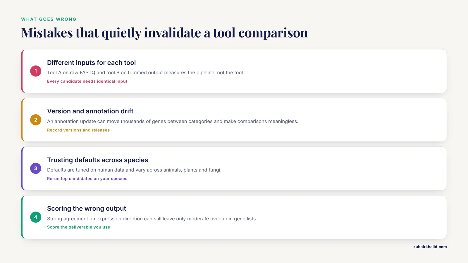
- Comparing tools on different inputs. Running tool A on raw FASTQ and tool B on the output of tool A's own trimming step measures the pipeline, not the tool. Every candidate must receive byte-identical input.
- Ignoring version and annotation drift. An annotation update can move thousands of genes between categories. The fungal pathogen reanalysis succeeded despite annotation version differences only because the team tracked and documented them explicitly [9]. Silent annotation swaps make comparisons meaningless.
- Trusting defaults across species. Defaults are usually tuned on human data. The multi-species workflow study found real performance variation across animals, plants, and fungi, and derived its species-specific recommendations from 288 tested pipelines rather than defaults [3].
- Scoring the wrong output. Two platforms can agree strongly on expression direction and still produce only moderate overlap in differential gene lists, as shown in the FFPE archival tissue comparison [10]. Score the deliverable, whether that is a gene list, an event table, or a cell label.
- Extending a benchmark past its design. Splicing tools that excel on standard short reads were still mostly unable to discover novel splice sites [1], and splicing tools that work on short reads can fail outright on long-amplicon protocols [2]. A winner on one data type is not a winner on yours until tested.
- Not planning for mixed or specialized samples. In dual RNA-seq, host-first mapping quietly discards pathogen signal, and pathogen-first mapping recovers more of it [7]. If your samples are mixtures, your comparison must include mapping order as a variable.
- Benchmarking with only one dataset. Single-dataset comparisons cannot separate tool effects from dataset quirks. Use at least two real datasets plus one simulation, and check that rankings are stable across them.
- Forgetting that benchmarks are arguments. Peer-reviewed comparisons draw critiques of their technical choices, as happened publicly with a T cell repertoire benchmark [5]. Defend your own choices in writing, and read others' benchmarks as claims to verify, not verdicts.
- Overfitting the simulation. If you tune the simulator until your preferred tool wins, you have built a mirror, not a benchmark. Use simulator settings that reflect real library preparation effects, such as the GC bias, hexamer priming, and barcode error modeling that BEERS2 implements [8], and always confirm the ranking on real data.
One final limitation deserves its own line. A tool comparison narrows your software risk, not your biological risk. Interpretation of the winning pipeline's output still requires domain expertise about your organism, tissue, and experimental design.
Frequently Asked Questions
What is the best bioinformatics software for RNA-seq differential expression?
There is no single best tool, because the answer depends on your species, library type, and experimental design. The defensible approach is to benchmark two or three candidates, such as DESeq2 and edgeR fed by two different counting strategies, on data where the right answer is known, and to pick the one that is both accurate and stable on your data.
How do I compare RNA-seq analysis tools step by step without an HPC cluster?
You can run a meaningful comparison on a 32 GB workstation for small datasets, using Conda for environment control and one or two samples per tool per condition. Use simulated or downsampled data for the accuracy runs, and borrow cluster time or a cloud instance only for the runtime and memory measurements, which are the resource-hungry part.
Do I need simulated data to compare RNA-seq tools?
For accuracy claims, yes. Simulation is the only setting where you know the correct answer for every read and every event, and modern simulators model realistic library effects down to GC bias and barcode errors. Real public data should complement simulation to confirm that the ranking holds under real bias, but simulation is what turns disagreement into a verdict.
Which tool should I use for alternative splicing analysis?
Independent benchmarks place SUPPA, DARTS, rMATS, and LeafCutter at the top of the event-based field for standard short-read data, with the best choice depending on whether you prioritize precision or recall. Match the tool to your read type as well, because rankings change on long-amplicon and targeted protocols.
How many datasets do I need for a fair comparison?
At minimum, one simulated dataset with a truth table plus two real datasets that differ in tissue or condition. If the ranking flips between real datasets, that instability is itself the finding, and you should report the tools as condition-dependent rather than declaring a universal winner.
Can I fairly compare an aligner-based tool with a pseudoalignment tool?
You cannot compare them directly, because they accept and produce different things, but you can compare their shared downstream output. Align both paths, feed each count or abundance matrix through the same differential expression model, and score the final gene lists against the same truth set.
How do I know a benchmark winner will work on my own data?
You do not, until you rerun the top candidates on a small slice of your own data with your own reference genome, annotation, and library type. Species, read protocol, and sample quality all shift tool rankings, so treat any published ranking as a shortlist rather than an answer.
Should I use AI or large language model tools for cell-type annotation in single-cell RNA-seq?
They are now serious candidates. Recent benchmarks show top LLM models outperforming traditional annotation methods, especially for fine-grained subtypes, with performance depending heavily on how marker genes are selected and ranked. Include them in your comparison the same way as any other tool, with a truth set and documented inputs, rather than adopting them on reputation.
Sources
- A comprehensive benchmarking of differential splicing tools for RNA-seq analysis at the event level.
- Computational Comparison of Differential Splicing Tools for Targeted RNA Long-Amplicon Sequencing (rLAS).
- A comprehensive workflow for optimizing RNA-seq data analysis.
- Optimizing bioinformatic workflows to extract clinically usable gene expression data from targeted tumor RNA sequencing panels: comparison with total RNA-seq in cancer samples.
- Comment on 'rigorous benchmarking of T cell receptor repertoire profiling methods for cancer RNA sequencing'.
- Split Pool Ligation-based Single-cell Transcriptome sequencing (SPLiT-seq) data processing pipeline comparison.
- Optimal Dual RNA-Seq Mapping for Accurate Pathogen Detection in Complex Eukaryotic Hosts.
- BEERS2: RNA-Seq simulation through high fidelity in silico modeling.
- Standardizing RNA-seq Analysis of Fungal Pathogens Using BRC-Analytics and Agentic AI: A Candidozyma auris Case Study.
- Strong correlation of gene counts and differentially expressed genes between a 3' RNA-Seq and an RNA hybridization platform in transcriptome analyses from canine archival tissues.
- Tool Comparison for Detecting Tumour Cells in Endometrial Cancer via Single-Cell Copy Number Variations Analysis.
- Benchmarking large language models for cell typing in single-cell RNA-Seq.