Reshaping Expression Data with pandas

By Dr. Zubair Khalid, DVM, MS, PhD · 2026-11-11

By the end of this article you will be able to take any gene expression matrix, whether it comes from an RNA-seq count table, a microarray scan, or a qPCR plate export, and convert it between wide format (one row per gene, one column per sample) and long format (one row per gene-sample observation) using pandas. You will learn the melt, pivot, pivot_table, stack, unstack, and transpose operations through a complete worked example, learn how to verify that a reshape preserved your data, and learn the exact error messages that appear when a reshape goes wrong and how to fix each one.

To follow along you need Python 3.9 or newer and pandas 1.5 or newer (the examples were checked against pandas 2.x behavior). Install pandas with pip install pandas. A Jupyter notebook is convenient but not required. Nothing else is mandatory, though the closing section touches on plotting and on Biopython for readers building larger pipelines.

Why Expression Data Needs Reshaping

Expression data lives in two shapes, and almost every downstream tool prefers one of them.

Wide format is the shape you get from featureCounts, Salmon, a GEO series matrix, or a limma object exported to CSV. Each row is a gene. Each column is a sample. A table with 20,000 genes and 12 samples occupies 20,000 rows and 12 data columns.

Long format (often called tidy format) has one row per measured value. The same 20,000 by 12 table becomes 240,000 rows with three columns: gene, sample, and expression value.

Neither shape is better. Wide format is compact and matches how most expression tools expect input. Long format matches how plotting libraries such as seaborn expect input, how groupby aggregations work naturally, and how you join sample metadata onto measurements. Reshaping expression data with pandas means moving between these two shapes without losing or duplicating a single number.

The pandas documentation describes melt as the operation that converts a DataFrame from wide to long, and pivot as its inverse. Those two functions, plus pivot_table for aggregation and stack/unstack for MultiIndex work, cover essentially every reshape you will perform in python for bioinformatics work.

Installing and Setting Up

python -m pip install pandas
python -m pip install jupyter   # optional but recommended

Check your versions before you start, because reshape behavior changed between pandas 1.x and 2.x in a few places:

import pandas as pd
print(pd.__version__)
# 2.2.3

Use the standard import alias. Every code block below assumes this line has run:

import pandas as pd

The Running Example: A Small Expression Matrix

Everything that follows uses one small, fully reproducible count matrix so you can paste the code and compare your output character for character. In real work you would load this from a file, which Step 1 also shows.

counts = pd.DataFrame(
    {
        "sample": ["tumor_1", "tumor_2", "normal_1", "normal_2"],
        "BRCA1": [512, 480, 95, 88],
        "TP53": [1300, 1410, 210, 190],
        "EGFR": [760, 715, 305, 288],
    }
).set_index("sample")

print(counts)

Expected output:

          BRCA1  TP53  EGFR
sample
tumor_1     512  1300   760
tumor_2     480  1410   715
normal_1     95   210   305
normal_2     88   190   288

This is classic wide format. Four samples in rows, three genes in columns. The sample names encode the biology: tumor_ versus normal_, with two replicates each. That naming convention is common in raw count files and becomes a problem the moment you want to group by condition, which is exactly why reshaping comes first in most expression workflows.

Reshaping Expression Data with pandas: Pivot and Melt Step by Step

This walkthrough covers reshape expression data pandas pivot melt step by step, moving from loading a real file through every major reshape operation.

Step 1: Load and Inspect the Count Matrix

Real expression data starts as a file. The most common layout is a CSV or TSV with gene identifiers in the first column:

counts = pd.read_csv(
    "counts.csv",
    index_col=0,        # use the first column (gene IDs) as the row index
)
print(counts.shape)
print(counts.dtypes)
print(counts.head())

Three checks matter before any reshape:

1. counts.shape should report (n_genes, n_samples). If the sample count is off by one, the gene ID column was treated as data, which means you forgot index_col=0.
2. counts.dtypes should show an integer or float dtype for every sample column. If a column shows object, the file contains a stray text value such as NA, null, or a hidden space, and pandas fell back to a generic object dtype. Fix that before reshaping, because melting an object column silently carries strings into downstream numeric code.
3. Confirm the index is unique with counts.index.is_unique. Duplicate gene identifiers will break the pivot step later, so it is far cheaper to catch them now.

If you are starting from the in-memory example instead, counts is already in the shape shown above and you can skip to Step 2.

Step 2: Melt the Matrix into Long Format

melt converts each gene-by-sample cell into its own row. The parameter that matters most is id_vars, the list of columns that stay put as identifiers. When the sample identifiers live in the index, as they do here, reset the index first so melt can see them as a regular column:

long = counts.reset_index().melt(
    id_vars="sample",       # columns to keep as identifiers
    var_name="gene",        # name for the former column headers
    value_name="counts",    # name for the values themselves
)

print(long.head(8))

Expected output:

     sample   gene  counts
0   tumor_1  BRCA1     512
1   tumor_2  BRCA1     480
2  normal_1  BRCA1      95
3  normal_2  BRCA1      88
4   tumor_1   TP53    1300
5   tumor_2   TP53    1410
6  normal_1   TP53     210
7  normal_2   TP53     190

Read this carefully, because it defines everything downstream. Each original cell became one row. The gene name, which was a column header, is now data in the gene column. The expression value is now data in the counts column. The output is sorted by gene first because melt processes one value column at a time, top to bottom.

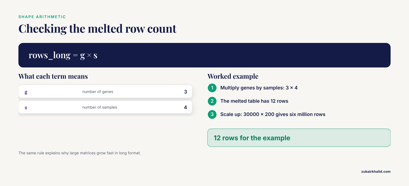
The shape relationship is worth memorizing. For a wide table of g genes and s samples, the melted table has exactly g × s rows. Here, 3 genes times 4 samples gives 12 rows:

print(long.shape)
# (12, 3)

Two melt parameters go unused in the simple case but matter in real files:

• value_vars restricts which columns get melted. If your file mixes count columns with annotation columns such as gene_length or gc_content, pass only the sample columns: value_vars=["tumor_1", "tumor_2", "normal_1", "normal_2"]. Anything not listed in value_vars and not in id_vars is dropped.
• Unnamed id_vars behavior changed across pandas versions. In every version, columns not named in id_vars and not in value_vars are discarded, which surprises people who expect melt to keep everything. Name your id_vars explicitly.

Step 3: Attach Sample Metadata in Long Format

The main payoff of long format is joining metadata. Suppose you have a design sheet:

metadata = pd.DataFrame(
    {
        "sample": ["tumor_1", "tumor_2", "normal_1", "normal_2"],
        "condition": ["tumor", "tumor", "normal", "normal"],
        "batch": ["A", "A", "B", "B"],
    }
)

long = long.merge(metadata, on="sample", how="left")
print(long.head())

Expected output:

     sample   gene  counts condition batch
0   tumor_1  BRCA1     512     tumor     A
1   tumor_2  BRCA1     480     tumor     A
2  normal_1  BRCA1      95    normal     B
3  normal_2  BRCA1      88    normal     B
4   tumor_1   TP53    1300     tumor     A

Now a groupby computes per-condition summaries in one line, something that is genuinely awkward in wide format:

print(long.groupby(["condition", "gene"])["counts"].mean().round(1))

Expected output:

condition  gene 
normal     BRCA1      91.5
           EGFR      296.5
           TP53      200.0
tumor      BRCA1     496.0
           EGFR      737.5
           TP53     1355.0
Name: counts, dtype: float64

This is the pattern behind most exploratory analysis of expression data: melt, join metadata, group, summarize.

Step 4: Pivot Back to Wide Format

pivot is the inverse of melt. It takes the gene column values and spreads them back out as column headers:

wide = long.pivot(
    index="sample",      # what becomes the row index
    columns="gene",      # what becomes the column headers
    values="counts",     # what fills the cells
)

print(wide)

Expected output:

gene      BRCA1  EGFR  TP53
sample                     
tumor_1     512   760  1300
tumor_2     480   715  1410
normal_1     95   305   210
normal_2     88   288   190

Notice two things. First, the column order changed because pivot sorts the new columns alphabetically. Second, the original index order was preserved on the rows. Column order rarely matters for analysis, but if a downstream tool expects the original order, restore it with wide = wide[counts.columns].

A full round trip should return your starting data exactly. That property becomes your verification tool later:

pd.testing.assert_frame_equal(
    wide[counts.columns], counts, check_exact=True
)

No output means success. An AssertionError here means the reshape lost or altered values.

Step 5: Aggregate Replicates with pivot_table

pivot refuses to average. If the same index-column pair appears more than once, it raises an error (shown in the errors section below). When your long table contains replicate measurements and you want one value per combination, use pivot_table, which aggregates:

long["condition"] = long["sample"].str.split("_").str[0]

wide_by_condition = long.pivot_table(
    index="gene",
    columns="condition",
    values="counts",
    aggfunc="mean",       # average across replicates
)

print(wide_by_condition.round(1))

Expected output:

condition  normal   tumor
gene                     
BRCA1         91.5   496.0
EGFR         296.5   737.5
TP53         200.0  1355.0

The aggfunc parameter accepts "mean", "median", "sum", "count", "max", or any callable. "count" is useful as a sanity check, because it shows how many replicates fed each cell. pivot_table also accepts fill_value to replace missing combinations (the default leaves them as NaN) and margins=True to append row and column totals, which is occasionally handy for QC on raw counts.

Step 6: Stack and Unstack for MultiIndex Data

stack and unstack are the compact, index-based versions of melt and pivot. They operate on the index rather than on named columns, which makes them the natural tools when your data already carries a MultiIndex.

stack pivots the columns into the index, producing a Series with a MultiIndex:

stacked = counts.stack()
print(stacked.head(6))

Expected output:

sample    gene 
tumor_1   BRCA1     512
          TP53     1300
          EGFR      760
tumor_2   BRCA1     480
          TP53     1410
          EGFR      715
dtype: int64

unstack does the reverse, pivoting one index level out into columns:

recovered = stacked.unstack()
pd.testing.assert_frame_equal(recovered[counts.columns], counts, check_exact=True)

These functions shine when you have hierarchical data, for example expression measured across two time points and three treatments:

index = pd.MultiIndex.from_tuples(
    [
        ("0h", "control"), ("0h", "treated"),
        ("6h", "control"), ("6h", "treated"),
    ],
    names=["time", "treatment"],
)

panel = pd.DataFrame(
    {"gene_A": [100, 150, 120, 400], "gene_B": [80, 90, 85, 210]},
    index=index,
)

print(panel.unstack("treatment"))

Expected output:

        gene_A          gene_B        
treatment control treated control treated
time                                          
0h            100     150      80      90
6h            120     400      85     210

One pandas 2.x detail worth knowing: starting with pandas 2.1, calling stack on a DataFrame with any missing values emits a FutureWarning recommending stack(future_stack=True). The new implementation never fills missing values silently, which is safer for expression data, where a missing cell usually means something went wrong upstream and should not be quietly converted to zero.

Step 7: Transpose for Heatmaps and Clustering

Transposing is the simplest reshape, and the one people forget. Seaborn clustermaps, hierarchical clustering, and many correlation routines want features in rows. Expression matrices usually already have genes in rows, but plotting libraries sometimes expect samples in rows instead:

import seaborn as sns  # pip install seaborn

counts_log = (counts + 1).apply(pd.np.log2) if False else None
# Simpler and dependency-free: use numpy directly
import numpy as np

log_counts = np.log2(counts + 1)      # +1 pseudocount avoids log2(0)
sns.clustermap(log_counts.T)          # samples as rows, genes as columns

counts.T swaps rows and columns in one call with no parameters to misconfigure. It is technically not a melt or pivot, but it belongs in any list of reshape expression data pandas pivot melt tips because half of all "why is my heatmap transposed" questions end here.

A Reference Table of Key Parameters

Keep this table next to your notebook until the calls become automatic.

Verifying That the Reshape Worked

Reshape bugs are silent by nature. The code runs, the output looks plausible, and a value quietly landed in the wrong sample. Three checks catch nearly every failure, and each takes one line.

Check 1: shape arithmetic. After melting a table with g rows and s value columns, the long table must have g × s rows:

n_values = counts.shape[0] * counts.shape[1]
assert long.shape[0] == n_values, "melt lost or duplicated rows"

Check 2: round trip. Melt then pivot, or stack then unstack, and assert equality against the original. This is the single strongest check because any misassignment of values breaks exact equality:

wide = long.pivot(index="sample", columns="gene", values="counts")
pd.testing.assert_frame_equal(wide[counts.columns], counts, check_exact=True)

The wide[counts.columns] reindexing handles the alphabetical column reordering that pivot introduces.

Check 3: observation counts. In long format, every gene should appear exactly s times and every sample exactly g times:

print(long["gene"].value_counts())
print(long["sample"].value_counts())

Expected output for the running example:

gene
BRCA1    4
TP53     4
EGFR     4
sample
tumor_1     3
tumor_2     3
normal_1    3
normal_2    3

Unequal counts mean the wide table had duplicate gene identifiers or that a sample column was dropped from value_vars by accident.

Common Errors and Exact Fixes

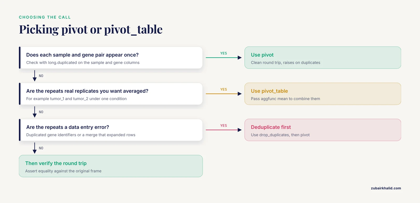
Reshape failures produce short, specific error messages. Here are the ones you will actually hit, with the message text and the fix.

ValueError: Index contains duplicate entries, cannot reshape. This is the most common pivot failure. It means the same index-column pair appears more than once in your long data, so pandas cannot decide which value goes in the cell. Typical causes are duplicated gene identifiers in the input file, melted annotation rows that duplicate the sample key, or a merge that expanded rows. Diagnose it directly:

dupes = long.duplicated(subset=["sample", "gene"], keep=False)
print(long[dupes].sort_values(["sample", "gene"]))

Then decide: deduplicate the input with drop_duplicates, or switch to pivot_table(aggfunc="mean") if the duplicates are legitimate replicates you intend to aggregate.

KeyError: 'gene'. pivot could not find a column you named. This almost always happens when the column you meant to use is actually sitting in the index, which is exactly the situation in Step 2 before the reset_index(). Check with print(long.columns) and print(long.index.name). If the name you need is in the index, call .reset_index() first or use stack/unstack, which operate on the index directly.

ValueError: cannot insert gene, already exists. You passed a var_name that collides with an existing column in the melted frame. Rename either the new column or the existing one before melting.

FutureWarning: The previous implementation of stack is deprecated and will be removed in a future version... Use stack(future_stack=True). Pandas 2.1 and later raise this on stack calls that would have involved dropping NaN values. Add future_stack=True to silence it and adopt the new behavior. The new implementation does not drop NaNs, so verify afterward with stacked.isna().sum() that you are not carrying unexpected missing cells forward.

SettingWithCopyWarning after reshaping. If you melted a slice such as counts.loc[:, sample_cols] and then assigned to the result, pandas may warn that you are writing to a copy. The values can still fail to persist in the original frame. The fix is explicit: build the slice with .copy(), for example counts.loc[:, sample_cols].copy(), before melting or modifying it.

A column of dtype object after loading. Not a reshape error, but it surfaces during reshape. melt will happily carry strings into your numeric column, and the first arithmetic operation downstream fails with something like TypeError: unsupported operand type(s) for +: 'int' and 'str'. Find the culprit rows with counts.applymap(lambda x: isinstance(x, str)).any() and clean them at load time with pd.read_csv(..., na_values=["NA", "null", "-"]).

Performance and Memory Tips

Real count matrices are large. A 30,000 gene by 200 sample matrix melted to long format produces six million rows, and naive handling can consume several times more memory than the wide original. Four practices keep reshaping fast.

Convert gene identifiers to categorical dtype after melting. A long table repeats each gene name tens or hundreds of times. Storing gene as category replaces those repeated strings with small integer codes:

long["gene"] = long["gene"].astype("category")

On a six-million-row table this alone typically cuts the memory footprint of the identifier column by a large factor, and groupby on categorical columns is faster as well.

Check memory before and after. long.info(memory_usage="deep") reports the true footprint including object strings. Run it before and after the categorical conversion so you know the conversion paid off.

Avoid chained reshapes in loops. Melting a large frame inside a per-gene loop is a common pattern in older scripts and a common source of hour-long runtimes. Melt once, then use groupby for all per-gene or per-sample work. The pandas documentation's grouping section describes vectorized groupby aggregation, which runs in compiled code rather than Python-level loops.

Consider the pyarrow-backed dtypes. In pandas 2.x you can load with pd.read_csv("counts.csv", index_col=0, dtype_backend="pyarrow"). Arrow-backed strings are far more compact than object strings, which helps when a metadata column forces melt to carry text alongside numeric values. This is an optional optimization, not a requirement, and it occasionally surfaces incompatibilities with older libraries, so test it on one file before adopting it across a pipeline.

Common Mistakes and Limitations

These are the mistakes that cost people the most time, stated plainly.

Melting annotation columns along with sample columns. If your count file includes gene_length, gc_content, or a gene symbol column, and you call melt with only id_vars="gene_id", those annotation columns get melted into the value column alongside the counts. The long table then mixes counts and gene lengths in one column, and every downstream mean is garbage. Pass sample columns explicitly in value_vars, or verify with long["gene"].value_counts() that the row count per gene equals the sample count.

Assuming pivot and pivot_table are interchangeable. pivot raises on duplicates. pivot_table silently averages them. If you reach for pivot_table out of habit when the data should have unique keys, you will average away a data-entry error instead of detecting it. Use pivot for clean round trips, pivot_table only where aggregation is the goal.

Trusting column order after a reshape. pivot sorts its new columns alphabetically and unstack sorts its new index level. Any code that assumes the original column order will misalign when you merge with another frame. Compare against named selections, never positional ones, and use df.reindex(columns=expected_order) when order matters.

Reshaping before joining metadata. Joining a metadata table onto a wide matrix by gene identifier is usually a mistake, because metadata describes samples, not genes. Join metadata in long format on the sample key, as Step 3 shows. Doing it in the wrong shape produces Cartesian merges that inflate row counts, which you can catch with the shape arithmetic check.

Letting NaNs disappear silently. The legacy stack dropped all-NaN rows by default, and pivot_table with a fill_value of 0 can turn a missing measurement into what looks like a zero count. Both behaviors destroy the distinction between "not measured" and "measured as zero." Decide explicitly how missing values should be handled and verify with isna().sum() after every reshape.

Forgetting that melt discards unnamed columns. Columns that are neither in id_vars nor value_vars are gone after the melt. If an annotation column vanished, that is why.

One limitation belongs in its own sentence. Reshaping is a mechanical step in a larger analysis, and the biological validity of your comparisons depends on normalization, batch handling, and study design decisions that individual cases need a qualified analyst or collaborator to review.

Where to Go Next

With the reshape in place, the standard next steps are a seaborn heatmap or clustermap on the transposed matrix, per-gene and per-sample QC summaries with groupby, and differential expression in a dedicated tool. If your pipeline needs to fetch gene annotations or sequences programmatically, the Biopython ecosystem is the usual companion to pandas in python for bioinformatics work, and a short biopython tutorial covering Bio.Entrez for NCBI queries pairs well with the metadata-joining pattern shown in Step 3. The pandas documentation's reshaping chapter, which covers melt, pivot, pivot_table, stack, and unstack with additional examples, is the authoritative reference for edge cases in your installed version, and its behavior notes for pandas 2.x explain the future_stack change described above.

Frequently Asked Questions

What is the difference between pivot and pivot_table in pandas?

pivot rearranges values without any computation and raises ValueError: Index contains duplicate entries, cannot reshape if the same index-column pair appears twice. pivot_table aggregates duplicates using aggfunc (mean by default), so it succeeds where pivot fails, at the cost of silently combining whatever it finds.

When should I melt expression data instead of keeping it wide?

Melt whenever you need to join sample metadata onto measurements, group by condition, batch, or time point, or plot with seaborn's long-format interface. Keep data wide for tools that expect a gene-by-sample matrix, such as most count-based differential expression inputs and heatmap functions.

How do I reshape a very large RNA-seq count matrix without running out of memory?

Melt only the sample columns with value_vars, convert identifier columns to category dtype immediately after melting, and inspect real memory use with info(memory_usage="deep"). For extremely large files, load with dtype_backend="pyarrow" in pandas 2.x or reshape in chunks and concatenate.

Why does pivot raise "Index contains duplicate entries, cannot reshape"?

Your long data has more than one row for the same index-column pair, most often because of duplicated gene identifiers or a merge that expanded rows. Find them with df.duplicated(subset=["index_col", "columns_col"], keep=False), then either deduplicate or switch to pivot_table with an appropriate aggfunc.

Can I melt several value columns at once, such as raw counts and TPM?

Yes. melt accepts multiple value columns and automatically creates one value_name column per value column, paired with the single var_name column. The result has one row per index-entry and value-column combination, so a table with two value columns produces two rows per gene-sample pair.

How should I handle missing values after melting or pivoting?

Decide explicitly rather than accepting a default. pivot_table fills absent combinations with NaN unless you pass fill_value, and pandas 2.1's stack(future_stack=True) preserves NaNs instead of dropping them. Count missing values with isna().sum() after every reshape, and only convert NaN to zero if a zero count is biologically meaningful for your assay.

Does melt preserve my original row and column order?

The identifier rows follow the order of the id_vars column, but the value columns are melted one at a time, so rows are grouped by the original column order rather than the original row order. If you need the original interleaving back after pivoting, reindex with df.reindex(columns=original_columns) or df.reindex(original_index).

Do I need Biopython for reshaping expression data?

No. Reshaping is pure pandas and Biopython adds nothing to melt or pivot. Biopython becomes relevant later in the workflow, for example when pulling gene annotations from NCBI to join onto your long-format expression table.