How to Assess the Reproducibility of a Bioinformatics Tool
By Dr. Zubair Khalid, DVM, MS, PhD ·

By the end of this article you will be able to take any bioinformatics tool, a versioned workflow engine, a container runtime, and a small reference dataset, and produce a quantitative reproducibility report: checksum-verified determinism, replicate concordance scores, parameter sensitivity ranges, and a provenance record that a reviewer can rerun. You will also know how to fold those numbers into a bioinformatics tools comparison when you must choose between candidate methods.
You need a Linux or macOS shell, Python 3, conda or mamba, Docker or Apptainer, R 4.x, bedtools, and a workflow engine such as Snakemake or Nextflow. All commands below run as written on a standard bioinformatics workstation.
What Reproducibility Means for a Bioinformatics Tool
The terms get used loosely, and the looseness causes real arguments between collaborators. Fix the vocabulary first. Repeatability means the same analyst reruns the same command on the same data on the same machine and gets the same numbers. Reproducibility, in the strict computational sense, means a different person on a different machine can rerun the analysis and get the same result. Replicability means running the same analysis design on new data and reaching the same conclusion. Kanwal's work on workflow reproducibility documents how much confusion surrounds these terms and how that confusion undermines attempts to verify published genomics analyses [1].
For genomics specifically, Baykal, Łabaj, Markowetz, and Mangul define genomic reproducibility as the ability of bioinformatics tools to maintain consistent results across technical replicates, and they argue this property, not just pipeline engineering, is central to validating biomedical discoveries [2]. That framing shifts attention to the tool itself. A pipeline can be perfectly containerized and versioned and still produce unstable output, because the tool inside the container is stochastic, sensitive to parameter choices, or dependent on a database that changes under it.
Assessing reproducibility of a bioinformatics tool therefore means answering five distinct questions:
- Is the tool deterministic on identical inputs?
- Is its output stable across technical replicates of the input data?
- How sensitive is the output to parameter perturbation?
- Does it behave identically across environments (conda, Docker, Apptainer, cluster)?
- Does the tool record enough provenance for a third party to rerun and audit it?
Each question has a concrete test, and the walkthrough below executes all five.
The Evidence That Tools Differ, and Why It Matters
Tool choice is not neutral. A benchmark of six recent cancer copy-number variation (CNV) callers on the hyper-diploid reference cancer genome HCC1395 found that copy gain, loss, and loss of heterozygosity calls were broadly consistent across sequencing centers, callers, and technologies, yet variation between callers was driven largely by how each tool estimated genome ploidy, with some software calling excessive gains or losses on a hyper-diploid genome [3]. The same study built a high-confidence call set by taking consensus across six callers and confirming with three orthogonal methods (microarray, Bionano, and sequencing) [3]. Two lessons carry directly into reproducibility assessment: tools disagree for identifiable mechanistic reasons, and consensus plus orthogonal validation is the standard remedy.
The dependence extends to the reference data a tool uses. In metagenomics, a systematic study of databases used to evaluate taxonomic classification and functional annotation tools found that tools are typically evaluated on dataset-specific bases, which makes direct comparison against state-of-the-art alternatives difficult, and that database choice determines whether a tool can resolve low-abundance species, distinguish closely related species, or handle high-diversity environmental samples [4]. A reproducibility assessment that ignores database version and composition is incomplete.
Preprocessing choices behave the same way. An analysis of patient clustering on 44 biomedical markers from the NHANES survey applied twelve combinations of preprocessing and clustering algorithms and evaluated the resulting clusters in an independent validation sample (1999 to 2002 for training, 2003 to 2006 for testing). Cluster quality and reproducibility of enrichment patterns differed across those combinations [5]. In other words, two pipelines that differ only in preprocessing can both be internally reproducible and yet produce different biology, which is why parameter sensitivity belongs in any serious assessment.
What You Need Installed
Run these checks before starting.
conda --version          # conda 23.x or later, or mamba
docker --version         # or apptainer --version
bedtools --version       # 2.30 or later
R --version | head -1    # 4.2 or later
snakemake --version      # 7.x or later
If a tool is missing, install through conda with the Bioconda channel, and prefer container images from the BioContainers Registry, which distributes more than 9,000 bioinformatics tools with standardized metadata, versions, and licenses for Conda, Docker, and Singularity formats [6]. Containerized distribution is not cosmetic. Docker-based registries built for bioinformatics, such as BioShaDock, exist precisely because containers provide process isolation and reproducibility across environments and versions, with domain-centric metadata from the EDAM ontology to make images findable [7]. Purpose-built distributions such as Dugong, an Ubuntu-based Docker image for bioinformatics, target reproducibility and replicability of entire analysis sessions [8].
Walkthrough: Assess a Tool in Nine Steps
This walkthrough uses a generic caller that produces genomic intervals (variant calls, peak calls, or CNV segments all fit the pattern). Substitute your tool and dataset. Every step produces a file you will keep.
Step 1. Freeze the Inputs
Compute checksums for every input file so you can prove later that inputs never changed.
mkdir -p repro_assessment/{data,results,logs}
md5sum data/* > results/input_checksums.md5
cat results/input_checksums.md5
Expected output:
3f5a8c0e91d2b7a6f4c1e8d2b7a6f4c1  data/sample.bam
9d2b7a6f4c1e8d2b7a6f4c1e8d2b7a6  data/reference.fa
...
Also record the reference database version the tool depends on. As the metagenomic database study shows, database identity is part of the tool's effective configuration, and evaluations done against different databases cannot be compared [4].
Step 2. Pin the Environment
Write a conda environment file with exact versions.
# env.yaml
name: repro-assess
channels:
  - conda-forge
  - bioconda
dependencies:
  - python=3.11
  - samtools=1.19.2
  - bedtools=2.31.1
  - r-base=4.3
conda env create -f env.yaml
conda activate repro-assessThen confirm the tool runs identically inside a container. Pull the tool's image from a curated registry rather than building an unpinned image, and record the image digest (the sha256: string printed by docker pull), because a tag alone can be moved.
docker pull biocontainers/yourtool@sha256:<paste-digest-from-registry>
docker run -v "$PWD":/work biocontainers/yourtool@sha256:<digest> \
  yourtool --version
Record both the conda solve and the container digest in your log. If the conda build and the container build of the same version produce different output at any later step, you have found an environment dependency the documentation did not disclose, which is itself a reproducibility finding.
Step 3. Test Bitwise Determinism
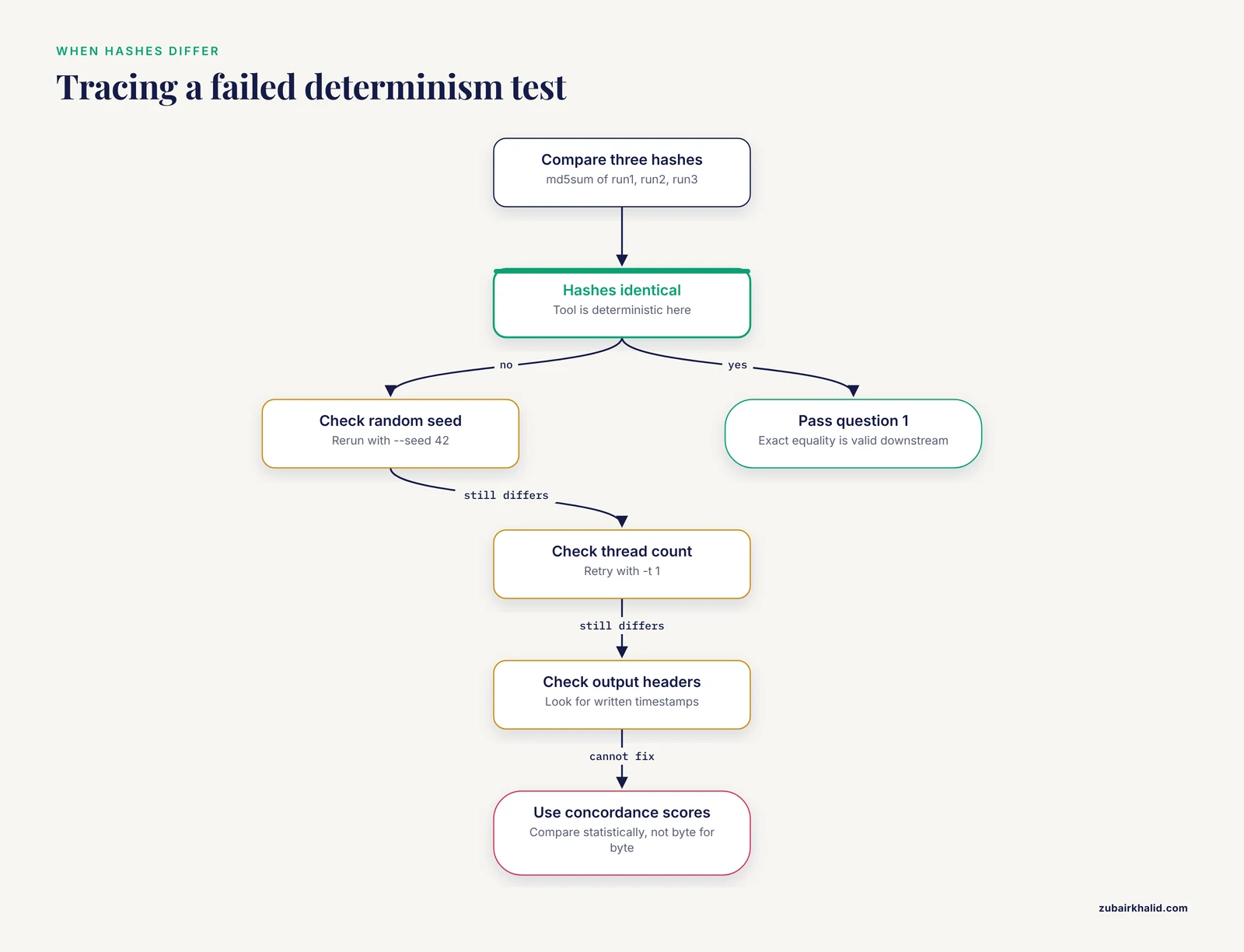
Run the tool three times on identical inputs with a fixed random seed (most callers expose a seed parameter), then compare outputs byte for byte.
for i in 1 2 3
do
  yourtool call -i data/sample.bam -o results/run$i.vcf --seed 42
done
md5sum results/run1.vcf results/run2.vcf results/run3.vcf
Expected output:
a1b2c3d4e5f6...  results/run1.vcf
a1b2c3d4e5f6...  results/run2.vcf
a1b2c3d4e5f6...  results/run3.vcf
Identical hashes mean the tool is deterministic under your configuration. If run3 differs, first check for unseeded randomness, multithreading with nondeterministic reduction order (try -t 1), or timestamps written into output headers. If you cannot force determinism, the tool fails question 1, and every downstream comparison must use statistical concordance rather than exact equality.
Step 4. Test Stability Across Technical Replicates
Deterministic on the same bytes is the easy test. The harder question is whether the tool's output is stable when the input data is resampled, which is what Baykal, Beerenwinkel, and Mangul address directly. Their method replaces biological replicates, which are a source of data variation, with synthetic replicates, runs the tool on the original data and on the synthetic replicates, and compares the outputs, revealing differences between results from original and synthetic data.
A practical synthetic replicate is a random downsampling of sequencing reads to a fixed fraction, generated with a fixed seed:
samtools view -s 0.50 -@ 4 data/sample.bam > results/synth50.bam
samtools view -s 0.75 -@ 4 data/sample.bam > results/synth75.bam
yourtool call -i results/synth50.bam -o results/synth50.vcf --seed 42
yourtool call -i results/synth75.bam -o results/synth75.vcf --seed 42
Here -s 0.50 retains roughly half the reads with a seeded random selection, and -@ 4 uses four threads. These downsampled files simulate independent technical replicates of the same library. The reproducibility question becomes: do the calls made on 50 percent and 75 percent of the data agree with the calls on 100 percent of the data?
Step 5. Score Concordance
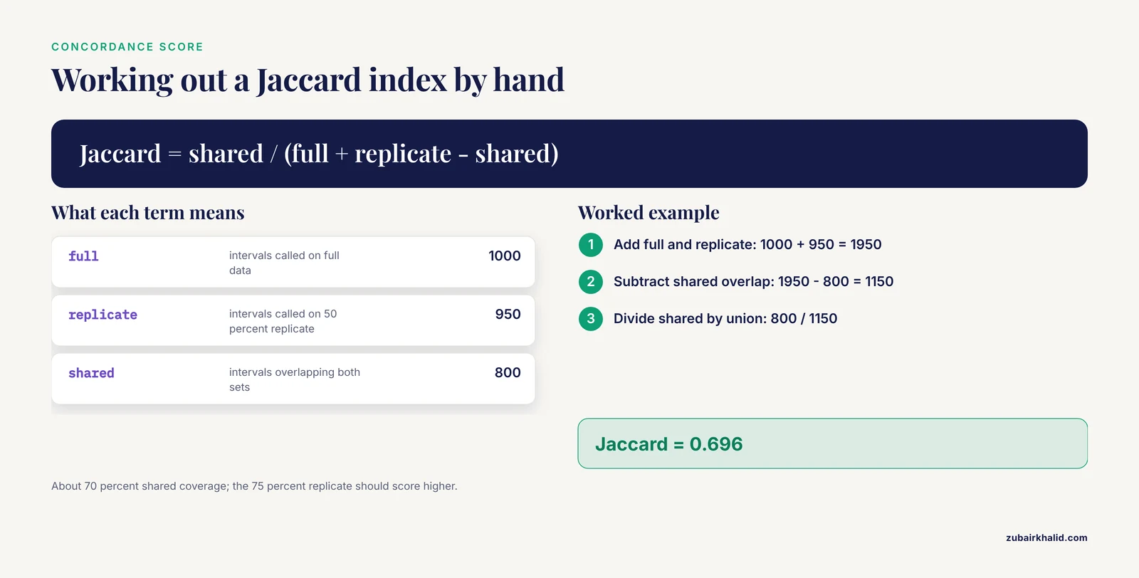
For interval outputs (CNV segments, peaks, variant clusters), use the Jaccard index, the size of the intersection divided by the size of the union of the two call sets. bedtools computes it directly:
bedtools sort -i results/run1.vcf > results/run1.sorted.bed
bedtools sort -i results/synth50.vcf > results/synth50.sorted.bed
bedtools jaccard -a results/run1.sorted.bed -b results/synth50.sorted.bed
Expected output:
intersection  union  jaccard
812           1136   0.7144
To see how the number is built, work one by hand. Suppose the full-data run calls 1,000 intervals, the 50 percent replicate calls 950, and 800 overlap. Then Jaccard = 800 / (1000 + 950 - 800) = 800 / 1150 = 0.696. Roughly 70 percent shared coverage. For the 75 percent replicate you would expect a higher value, and a tool whose Jaccard against a 75 percent replicate is still below about 0.5 is producing calls that are not anchored in the data.
For per-base or per-gene quantities (coverage, counts, expression), measure rank concordance in R:
run1 <- read.delim("results/coverage_run1.tsv")
syn50 <- read.delim("results/coverage_synth50.tsv")
m <- merge(run1, syn50, by = "feature")
cor.test(m$depth.x, m$depth.y, method = "spearman")
Expected output:
        Spearman's rank correlation rho

data:  m$depth.x and m$depth.y
S = 1.2e+09, p-value < 2.2e-16
rho = 0.94
Report rho for each replicate level. A tool is analytically stable when rho stays high as input shrinks and the Jaccard index degrades gracefully rather than collapsing.
Step 6. Test Parameter Sensitivity
Run the tool across a small grid of its two or three most consequential parameters, the ones the manual flags as model or threshold settings, and score each grid point against the baseline. Automate with Snakemake so every combination is recorded:
# Snakefile
PARAMS = [1, 2, 4, 8]

rule all:
    input: expand("results/p{p}/calls.vcf", p=PARAMS)

rule call:
    input: "data/sample.bam"
    output: "results/p{p}/calls.vcf"
    shell:
        "mkdir -p results/p{wildcards.p} && "
        "yourtool call -i {input} -o {output} "
        "-L {wildcards.p} --seed 42"
snakemake --cores 4
for p in 1 2 4 8
do
bedtools jaccard -a results/run1.sorted.bed \
-b <(bedtools sort -i results/p$p/calls.vcf) \
| awk -v p=$p 'NR>1 {print p, $3}'
doneExpected output:
1 1.000
2 0.913
4 0.842
8 0.701
A reproducible tool shows a smooth gradient, not cliffs. If one unit change in a parameter deletes half the calls, any published result from that tool is conditional on a setting nobody reported. The CNV benchmark illustrates the failure mode at the biological level: callers that mis-estimated ploidy on the hyper-diploid HCC1395 genome produced excessive copy gain or loss calls, so a single embedded model assumption changed the output dramatically [3].
Step 7. Test Portability Across Environments
Repeat steps 3 through 6 in the container and, if available, on a second platform (a cluster with Apptainer, or a collaborator's machine). Compute the same Jaccard and Spearman metrics between environments.
docker run -v "$PWD":/work \
  biocontainers/yourtool@sha256:<digest> \
  yourtool call -i /work/data/sample.bam \
  -o /work/results/docker_run1.vcf --seed 42
bedtools jaccard -a results/run1.sorted.bed \
                 -b <(bedtools sort -i results/docker_run1.vcf)
If conda and Docker builds of the same version disagree, diff the tool's own reported version and dependency list in both environments (yourtool, version, conda list) and record the divergence. Version drift between "the same" tool on two machines is one of the most common reproducibility failures, and container registries with standardized metadata exist specifically to prevent it [6], [7].
Step 8. Check Provenance Support
Provenance is the recorded chain of inputs, parameters, software versions, and steps that produced a result. A tool that records provenance automatically lets you reconstruct any output after the fact. Three concrete standards and tools to check for:
- QIIME 2's Provenance Replay generates new executable code from results the platform produced, closing the gap between a result file and the commands that created it, and the authors explicitly frame automated provenance tracking as the developer's responsibility for removing reproducibility barriers [10].
- BioCompute Objects (BCOs) provide a standardized, FAIR-compliant reporting structure for high-throughput sequencing workflows, encapsulating tools, platforms, datasets, and workflows, with support from cloud platforms including Galaxy, the Cancer Genomics Cloud, and HIVE [11].
- CoPaLink addresses the gap between what a paper says and what the code does, linking tool mentions in workflow code to tool mentions in the published description using named entity recognition and embedding-based entity resolution, with individual component F1 measures between 77 and 90 and a joint accuracy of 66 on Nextflow workflows [12].
Practical checks on your tool: does it write a version string and full command line into its output headers, does it emit a machine-readable run log, and can its output be replayed into a workflow engine without manual archaeology? If the answer to all three is no, plan to wrap the tool in a workflow system yourself and treat the wrapper, not the tool, as the reproducible unit. The reproducibility literature repeatedly identifies workflows as the practical unit of reproducible genomics analysis [1], and linking narrative method descriptions to workflow implementations is an active, only partially solved research problem [12].
Step 9. Write the Reproducibility Report
Assemble everything into a single document using the template in the next section. This is the deliverable a reviewer, a collaborator, or your future self actually reads.
A Reusable Reproducibility Report Template
Use this format verbatim. It doubles as a checklist, and filling every field forces you to complete the assessment.
# Reproducibility Assessment: <tool name>

## 1. Identity
- Tool and exact version:
- Container image and digest:
- Conda environment file: env.yaml (attached)
- Reference database name and version:
- Assessment date and hostname:

## 2. Inputs
- Dataset description:
- input_checksums.md5 (attached)
- Fixed random seed(s) used:

## 3. Determinism (Step 3)
- Repeat runs: 3
- Output md5sums identical: yes / no
- If no, suspected cause (threads, RNG, timestamps):

## 4. Replicate Stability (Steps 4-5)
- Synthetic replicate fractions tested: 0.50, 0.75
- Jaccard vs full data: 0.50x = __, 0.75x = __
- Spearman rho vs full data: 0.50x = __, 0.75x = __

## 5. Parameter Sensitivity (Step 6)
- Parameters varied and range:
- Jaccard per grid point: (list)
- Cliff detected: yes / no

## 6. Portability (Step 7)
- Environments compared: conda, docker, cluster
- Cross-environment Jaccard: __
- Divergences found: (describe)

## 7. Provenance (Step 8)
- Version and command line embedded in output: yes / no
- Machine-readable run log: yes / no
- Replayable in workflow engine: yes / no
- BCO or equivalent record exported: yes / no

## 8. Verdict
- Reproducible under stated conditions: yes / conditional / no
- Conditions and caveats:
This template is deliberately environment-agnostic. It matches the practice taught in graduate-level reproducibility training, where students learn versioning, containerization, and workflow systems and then apply them by reanalyzing a previously published study over several months, an exercise that reliably exposes how much effort real reproducibility takes [13].
Using the Assessment in a Bioinformatics Tools Comparison
When two or more candidate tools must be compared, run the same nine-step assessment on each and put the metrics side by side. This is the honest core of any bioinformatics tools comparison, and it aligns with how comparative reviews are structured. The cancer bioinformatics resource review by Saini and colleagues distinguishes databases, analytical web servers, prediction tools, and integrated platforms, and evaluates them along data coverage, analytical capabilities, evidence strength, limitations, and appropriate use cases [14]. That same multi-axis structure, with reproducibility metrics added, beats single-number rankings. Reviews of molecular typing resources for Mycobacterium tuberculosis reach the same conclusion from the pathogen genomics side, providing comprehensive tool and database comparisons specifically to guide selection while noting the reproducibility advantages of newer whole-genome methods over older typing approaches [15].
A comparison table worth publishing looks like this:
| Property | Test | Metric | What good looks like |
|---|---|---|---|
| , - | , - | , - | , - |
| Determinism | 3 identical runs, fixed seed | md5sum equality | Identical hashes |
| Replicate stability | Synthetic replicates [9] | Jaccard, Spearman rho | Graceful degradation, rho stays high |
| Parameter sensitivity | Small parameter grid | Jaccard vs baseline | Smooth gradient, no cliffs |
| Portability | Conda vs container vs cluster | Cross-environment Jaccard | Near 1.0 |
| Accuracy | Truth set or orthogonal methods [3] | Precision, recall, F1 | High and stable across conditions |
| Provenance | Output inspection [10], [11] | Replayability check | Full command line and versions embedded |
| Database fit | Versioned reference data [4] | Documented database identity | Explicit, pinned, citable |
When the goal is choosing the best bioinformatics software for a project, weight the reproducibility columns at least as heavily as headline accuracy. A tool with slightly lower accuracy but flat parameter sensitivity and full provenance will produce more reliable science over a project's lifetime than a marginally more accurate tool that swings with every setting change. For teams working in R, note that the language's ecosystem, from Bioconductor packages to R Markdown for literate analysis, has been a deliberate driver of reproducibility in statistical genomics [16]. For teams building infrastructure rather than analyses, container registries with FAIR metadata [6] and shared Docker-based registries with ontology-based tagging [7] are the current community answer to distribution-related reproducibility failures, and structured reporting standards such as BioCompute Objects make the resulting records interoperable across academic, industrial, and regulatory settings [11]. Early work on reproducible research practices in cancer bioinformatics by Carey and Stodden laid out these principles, separating concepts from concrete tooling, and the field has largely converged on the practices they described [17].
Common Mistakes and Limitations
Confusing a working rerun with reproducibility. If your own rerun succeeds on your own machine with your own cached files, you have tested nothing about reproducibility. The test only means something across environments, users, or resampled data.
Running the assessment on curated test data only. Tools often look stable on the small, clean example bundled with the distribution. Include at least one challenging, biologically atypical sample. The CNV benchmark chose a hyper-diploid genome deliberately, and that choice is what exposed the ploidy-estimation failures [3].
Ignoring random seeds and thread counts. Many tools are only deterministic at one thread. Assess determinism both single-threaded and at your production thread count, and report both.
Comparing tools evaluated on different databases. A metagenomic classifier tuned and scored against one database cannot be compared to another scored against a different one, and the database study shows this practice systematically obscures real performance differences [4]. Pin and report the database in every cell of a comparison.
Treating preprocessing as neutral. The NHANES clustering study showed that preprocessing and algorithm combinations change both cluster quality and reproducibility [5]. When you compare tools, hold preprocessing fixed or vary it explicitly as a factor.
Mistaking reproducibility for correctness. A tool can reproduce its own wrong answer perfectly. That is why the walkthrough includes a benchmark step against a truth set or orthogonal technologies, following the consensus-plus-validation design used in the CNV study [3]. Reproducibility is necessary, not sufficient, for validity.
Skipping provenance until publication time. Retrofitting provenance from terminal history is slow and error-prone. Export provenance records (QIIME 2 Provenance Replay style [10], BCO [11]) at run time, and link your workflow code to the method text so others can map narrative claims to executable steps [12].
Overgeneralizing one assessment. Your results are conditional on your data type, genome, and parameter range. State the conditions in the verdict field of the template. Also budget real time for this work. Teaching experience from reproducibility-focused courses shows that implementing reproducible analyses is a complex task requiring significant effort [13].
Frequently Asked Questions
What is the difference between reproducibility and replicability in bioinformatics?
Reproducibility means a different person can rerun the same analysis on the same data and get the same result, while replicability means running the same analysis design on new data and reaching the same conclusion. For genomics tools specifically, a widely used working definition is consistency of results across technical replicates [2], [1].
How do I test the stability of a tool when I have only one sample?
Replace biological replicates with synthetic replicates. Generate synthetic replicates, for example by seeded downsampling of reads, run the tool on the original data and on the synthetic replicates, and compare the outputs quantitatively.
What Jaccard index or correlation value means a tool is reproducible?
There is no universal threshold. Interpret the metric relative to the perturbation: concordance should degrade gradually as input is downsampled or parameters shift, and a collapse from near 1.0 to below 0.5 across a small change signals instability. Always report the conditions alongside the number.
Can a tool be perfectly reproducible and still give wrong results?
Yes. Determinism and replicate stability say nothing about accuracy, which is why an assessment must include a benchmark against a truth set or orthogonal methods, as done in the six-caller CNV study that validated calls with microarray and Bionano data [3].
Do containers guarantee reproducibility?
No. Containers fix the software environment, which removes a whole class of version drift and installation failures [7], [8], but they do not fix unseeded randomness, database changes, or parameter sensitivity. Containerize and then run the full assessment.
What is the fastest sanity check that a published analysis is reproducible?
Check three things: whether code and exact software versions are available, whether inputs and reference databases are pinned and identifiable, and whether the workflow can be replayed with a standard engine. Tools that automatically capture provenance, such as QIIME 2's Provenance Replay, make this check nearly instant for results produced within that platform [10].
How should reproducibility be reported in a methods section?
Use a structured record rather than prose alone. A BioCompute Object captures workflow, data, provenance, and validation information in a FAIR-compliant format supported by platforms including Galaxy and the Cancer Genomics Cloud [11], and a filled-in reproducibility report template covering determinism, stability, sensitivity, portability, and provenance is the practical minimum.
Which tools qualify as the best bioinformatics software for reproducible work?
There is no single best tool, only the best fit. Evaluate candidates with the same comparison table: accuracy against a truth set, replicate stability, parameter sensitivity, environment portability, container availability from a curated registry [6], and automatic provenance support [10]. Comparative reviews of domain resources recommend exactly this multi-axis evaluation over single-number rankings [14].
Sources
- Understanding reproducibility of bioinformatics workflows
- Genomic reproducibility in the bioinformatics era
- Evaluation of somatic copy number variation detection by NGS technologies and bioinformatics tools on a hyper-diploid cancer genome
- A comprehensive study of databases to assess the reliability of metagenomic tools
- Unsupervised Analysis of Classical Biomedical Markers: Robustness and Medical Relevance of Patient Clustering Using Bioinformatics Tools
- BioContainers Registry: searching bioinformatics and proteomics tools, packages, and containers
- BioShaDock: a community driven bioinformatics shared Docker-based tools registry
- Dugong: a Docker image, based on Ubuntu Linux, focused on reproducibility and replicability for bioinformatics analyses
- Reproducibility of Bioinformatics Tools
- Facilitating bioinformatics reproducibility with QIIME 2 Provenance Replay
- Bioinformatics tools developed to support BioCompute Objects
- Supporting workflow reproducibility by linking bioinformatics tools across papers and executable code
- Reprohackathons: promoting reproducibility in bioinformatics through training
- Web servers and bioinformatics tools for cancer research: A review.
- Molecular typing of Mycobacterium tuberculosis: a review of current methods, databases, softwares, and analytical tools
- The R Language: An Engine for Bioinformatics and Data Science
- Reproducible Research Concepts and Tools for Cancer Bioinformatics