How to Read a FASTA File in R
By Dr. Zubair Khalid, DVM, MS, PhD ·

By the end of this article you will be able to import a FASTA file into R, inspect the sequence names and lengths, compute basic statistics such as total bases and GC content, extract a subset of records, and write the result back to disk as a valid FASTA file. You will also know which R package to pick for a given file size and how to diagnose the errors that come up most often when reading sequence data.
To follow along you need R installed (version 4.0 or newer is a sensible baseline), the ability to install packages from CRAN and Bioconductor, and a FASTA file to work with. If you do not have one, any nucleotide or protein FASTA downloaded from a sequence database will do. The examples below use a small toy file so you can verify every output on your own machine.
FASTA is the de facto exchange format for raw sequence data in genomics. Researchers use it everywhere, from defining target regions for adaptive sampling on long-read sequencers, where a simple specification of the target region in a FASTA file tells the instrument whether a DNA fragment should be sequenced [1], to building merged reference genomes for resequencing projects [2]. Reading it correctly is the first step in almost every R for bioinformatics workflow you will ever run.
What a FASTA File Actually Contains
A FASTA file is plain text made of repeating blocks. Each block starts with a header line that begins with a greater-than character, followed by a sequence identifier and usually a description. The lines after the header contain the sequence itself, typically wrapped at 60 or 80 characters, although the wrapping width is not guaranteed by the format.
Here is a three-record nucleotide FASTA file we will call toy.fasta:
>seq1 description here
ATGCGTACGTAGCTAGCTAG
GCTAGCTAGCTAG
>seq2 another record
ATGGCGCGTATGCGCGATCG
TTAGCGCGCGAT
>seq3 third record
GGCCTTAAGGCCTTAAGGCC
TTAAGGCC
Three details of the format matter when you parse it in R:
- Every header line starts with
>. Anything after the first whitespace character on that line is a free-text description. - A sequence can span any number of lines. Newlines inside a sequence carry no biological meaning, so a parser must concatenate them.
- A single file can hold one record or millions. The multi-record form is called multi-fasta, and tools that merge such files must preserve the boundaries between the original sequences so downstream analyses can still tell which genome a read came from [2].
The format also has standardized extensions. The Proteomics Standards Initiative defined an extended FASTA format, called PEFF, that adds controlled mechanisms for encoding metadata such as sequence variants and post-translational modifications while remaining nearly backward compatible, so standard FASTA parsers can read PEFF files as ordinary FASTA files [3]. You will rarely need to handle PEFF explicitly in R, but you should know it exists when someone hands you a proteomics database export.
Finally, do not confuse a sequence FASTA file with a FASTA output file from a local similarity search. Search tools produce alignment reports that are far more complex to parse, and the research community has built dedicated graphical tools precisely because those reports are painful to read in a text editor [4]. This article is about sequence files, not search outputs.
Setup: Installing R and Bioconductor Packages
Bioconductor is a collection of open source, open development packages for the R programming language, widely used for genomics data analysis [5]. Most serious sequence-file work in R goes through Bioconductor packages, so set that repository up first.
Install Bioconductor's package manager and then install Biostrings, the core package for sequence containers:
install.packages("BiocManager")
BiocManager::install("Biostrings")
For indexing large files you will also want Rsamtools, and for format conversion work seqinr is a useful companion from CRAN:
BiocManager::install("Rsamtools")
install.packages("seqinr")
If you later need to convert between GenBank, EMBL, FASTA, and other sequence formats, note that standalone command-line tools such as Readseq have handled this job for decades and can read and write many different formats [6]. R is one option among several, and sometimes the right move is to convert the file before R ever sees it.
Method 1: Reading FASTA with Biostrings (Recommended)
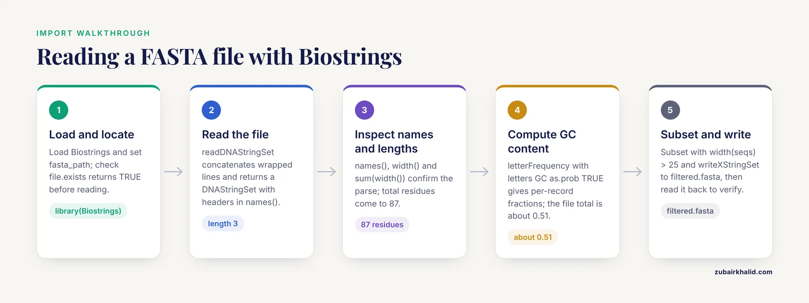
Biostrings is the Bioconductor package for storing biological sequences efficiently in memory. Its reader functions are fast, validated, and handle the line-wrapping problem for you. This is the method to learn first.
Step 1: Load the package and point to your file
library(Biostrings)

fasta_path <- "toy.fasta"
Use an absolute path or set your working directory with setwd() so the relative path resolves. A common sanity check is file.exists(fasta_path), which should return TRUE before you attempt anything else.
Step 2: Read the file
seqs <- readDNAStringSet(fasta_path)
seqs
Expected output for toy.fasta:
DNAStringSet object of length 3:
    width seq                                           names
[7]    32 ATGCGTACGTAGCTAGCTAGGCTAGCTAGCTAG             seq1 description here
[1]    31 ATGGCGCGTATGCGCGATCGTTAGCGCGCGAT              seq2 another record
[3]    24 GGCCTTAAGGCCTTAAGGCCTTAAGGCC                  seq3 third record
The reader found all three records, concatenated the wrapped lines, and returned an object of class DNAStringSet. The names() attribute holds the full header text after the >, descriptions included.
Step 3: Inspect names and lengths
names(seqs)
width(seqs)
sum(width(seqs))
names(seqs) returns the three headers as a character vector. width(seqs) returns the per-record lengths, here 32, 31, and 24. sum(width(seqs)) gives the total number of residues, 87 in this example. These three calls are the quickest way to confirm the file parsed as expected.
Step 4: Compute basic statistics
letterFrequency(seqs, letters = "GC", as.prob = TRUE)This returns a matrix with one row per record and one column giving the fraction of G and C residues. To get the GC content of the whole file:
gc_total <- sum(letterFrequency(seqs, letters = "GC"))
all_total <- sum(width(seqs))
gc_total / all_total
For toy.fasta this evaluates to about 0.51, which you can verify by hand against the sequences above.
Step 5: Extract and subset
seqs[7]
seqs["seq2"]
seqs[width(seqs) > 25]
Biostrings objects support standard R subsetting. The second line uses the name directly, which works when every header is unique.
Step 6: Write results back to FASTA
writeXStringSet(seqs[width(seqs) > 25], "filtered.fasta")This produces a valid FASTA file containing only the records longer than 25 residues, with sequences rewrapped at a standard width. Rounding-tripping your data through writeXStringSet and reading it back in is a good habit during pipeline development.
Choosing the right reader function
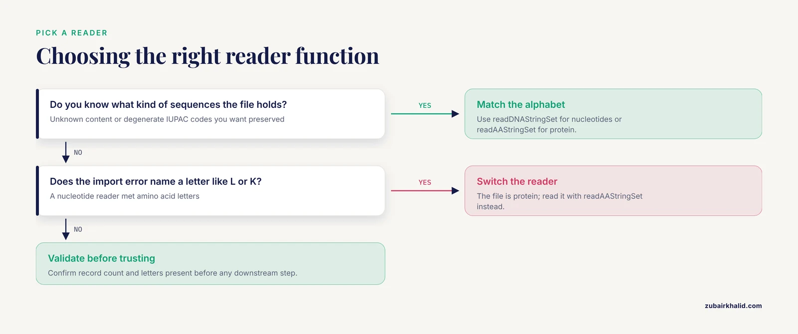
Biostrings provides a family of readers matched to sequence type:
readDNAStringSet()   # nucleotide sequences
readRNAStringSet()   # RNA sequences
readAAStringSet()    # amino acid (protein) sequences
readBStringSet()     # raw bytes, no alphabet checking
If you read protein data with readDNAStringSet(), the function will error as soon as it encounters an amino acid letter outside the DNA alphabet. When you are unsure what a file contains, or when it contains degenerate IUPAC codes you want preserved without validation, use readBStringSet() first and inspect it before committing to a stricter class.
Method 2: Reading FASTA with seqinr
The seqinr package from CRAN is older than Biostrings but still widely used in teaching and in scripts that need lightweight sequence manipulation. Its reader works differently and returns an R list rather than a Bioconductor object.
library(seqinr)
seqs <- read.fasta("toy.fasta", seqtype = "DNA", as.string = FALSE)
Parameters worth knowing:
seqtypetells the parser whether to expect nucleotide or protein letters. It affects internal validation, not the raw text it reads.as.string = FALSEreturns each sequence as a character vector with one letter per element, which suits positional operations such asseqs[][1:10]. Settingas.string = TRUEreturns each sequence as a single character string instead.forceToLowercontrols case normalization and is on by default.
Inspect the result:
length(seqs)
names(seqs)
seqs[[7]][1:10]
getSequence(seqs[[7]], as.string = TRUE)
getAnnot(seqs[[7]])
getAnnot() extracts the description part of the header, which seqinr keeps separate from the identifier. This split is convenient when headers carry structured metadata you want to parse into a table later.
The trade-off against Biostrings is performance and scale. seqinr stores sequences as ordinary R character objects, which costs more memory per residue than Biostrings' compact encoding. For a few hundred or a few thousand records the difference does not matter. For a genome-sized file it does.
Method 3: Manual Parsing with Base R
Sometimes you need full control over parsing, for example when headers contain structured fields you want to split into columns, or when you want to understand exactly what a reader function does. The pattern below is the one to know.
lines <- readLines("toy.fasta")

is_header <- startsWith(lines, ">")
ids <- sub("^>(\\S+)", "\\1", lines[is_header])
descriptions <- sub("^>\\S+\\s*", "", lines[is_header])
descriptions[descriptions == ""] <- NA_character_

seq_lines <- split(lines[!is_header], rep(seq_along(ids), times = diff(c(which(is_header), length(lines) + 1))))
sequences <- sapply(seq_lines, paste, collapse = "")
Walk through what each line does:
readLines()reads the whole file into a character vector, one element per line.startsWith(lines, ">")identifies header lines by their first character, which is the only reliable rule the format guarantees.- The first
sub()call keeps everything up to the first whitespace as the identifier. The second extracts the description, turning an empty description intoNA. - Sequence lines are grouped between consecutive header positions and collapsed into single strings, which correctly handles arbitrary line wrapping.
You can then build a data frame:
fasta_df <- data.frame(
  id = ids,
  description = descriptions,
  sequence = sequences,
  length = nchar(sequences),
  stringsAsFactors = FALSE
)
fasta_df
Expected output:
    id      description        sequence length
1 seq1  description here ATGCGTACGTAG...     32
2 seq2   another record  ATGGCGCGTAT...     31
3 seq3    third record   GGCCTTAAGGCC...     24
This approach is memory hungry because every line and every sequence string exists as an R object. It is appropriate for files up to tens of megabytes. For anything larger, use the indexed approach in the next section.
Comparing the Three Methods
| Criterion | Biostrings | seqinr | Base R manual parse |
|---|---|---|---|
| Install source | Bioconductor | CRAN | None needed |
| Returned object | DNAStringSet or similar | List of character vectors | Data frame you build |
| Alphabet validation | Yes, per class | Configurable | None |
| Memory efficiency | High (compact encoding) | Moderate | Low |
| Handles gzip directly | Yes, with Rsamtools or transparently by path | Limited | No |
| Best use case | Pipelines, large files, subsetting | Teaching, quick scripts, header annotation | Custom header parsing, full control |
For most readers, the answer to how to read a FASTA file in R is Biostrings. The other two methods earn their place when the job calls for their specific strengths.
Working with Large FASTA Files
Genome-scale FASTA files change the calculus. A human genome assembly in FASTA runs to several gigabytes uncompressed, and reference collections for metagenomics can be larger still. Two strategies matter here.
Random access with indexed files
The Rsamtools package creates a companion index file so you can pull individual records without loading the whole file:
library(Rsamtools)
library(Biostrings)

fa <- FaFile("genome.fasta")
indexFa(fa)                       # creates genome.fasta.fai, run once
seqinfo(fa)                       # inspect sequence names and lengths
fetch <- scanFa(fa, param = GRanges("chr1", IRanges(1000, 2000)))
The index records the byte offset of every record, which turns random access into a seek operation instead of a full-file scan. This is the same indexing scheme that alignment tools rely on, and it is the standard way to handle a reference genome in an R script that only needs a few regions.
Understanding parsing performance
File parsing itself can dominate runtime for I/O-heavy applications. Performance engineering work on FASTA and FASTQ parsing has shown how much speed is left on the table when tools read these files naively. The RabbitFX framework, designed for modern multi-core platforms, delivered speedups of at least 11.6-fold on plain files and 6.6-fold on gzip-compressed files when integrated into the quality-trimming tool fastp, with similar gains in two other I/O-intensive applications [7]. The lesson for R users is indirect but practical: parsing cost scales with file size and compression, so avoid re-reading the same large FASTA file repeatedly inside loops, prefer indexed access when you need only some records, and keep expensive parsing work outside per-iteration code.
Compression is a related decision. A gzip-compressed FASTA file saves disk space and network transfer time, and Biostrings accepts the .fasta.gz path directly in recent versions. The trade-off, reflected in the parsing benchmarks above, is that compressed input costs CPU time on every read [7]. If your script opens the same compressed file many times, decompressing it once to a temporary plain-text file and reading that repeatedly can be faster overall.
Chunked reading pattern
When you must process every record of a very large file but cannot hold it all in memory, iterate in batches. With Biostrings you can use FaFile indexing to walk through records by name ranges, or split the file upstream with standard command-line tools and process the chunks in R. The key principle is that no step should require the full uncompressed file in memory at once unless your machine genuinely has room for it.
Validating That Your Import Is Correct
Reading a file is only useful if the result is right. Four checks catch nearly every real-world problem:
- Record count. Count the headers in the raw file and compare with the object length:
sum(startsWith(readLines("toy.fasta"), ">"))
length(seqs)- Length distribution. Inspect
width(seqs)for zero-length records, which usually indicate a stray>line or a truncated file at the end.
- Alphabet. With Biostrings, ask which letters appear:
unique(ascii(unlist(strsplit(as.character(seqs[7]), ""))))Or more simply for the whole set:
sort(unique(unlist(strsplit(paste(sequences, collapse = ""), ""))))For nucleotide data you expect the IUPAC letters A, C, G, T, and possibly N plus ambiguity codes. A surprise letter such as a hyphen, a space, or a digit signals a malformed record or a different file type than you assumed.
- Round trip. Write the object out, read it back, and compare lengths and names. If
identical(width(original), width(reimported))isTRUEand the name vectors match, your pipeline stage did not silently corrupt anything.
Also confirm the sequence type matches your downstream tools. A protein FASTA read as DNA will fail loudly in Biostrings, which is helpful. Base R parsing will not complain at all, which is exactly why the alphabet check above earns its place.
Common Mistakes and Limitations
These are the errors that show up again and again when people first read FASTA files in R, together with their exact symptoms and fixes.
- Using
read.table()orread.csv()on a FASTA file. These functions assume delimited tabular data. A FASTA file has no consistent column count, soread.table()throws errors such as "line X did not have Y elements" or, worse, silently produces garbage. Use a dedicated reader or the manual parser above.
- Assuming one sequence per file. Many tutorials show single-record examples, so beginners write code that reads
sequences[7]and stops. Production FASTA files are multi-record almost by default, as the merging tools for multi-fasta reference genomes illustrate [2]. Always checklength()on the imported object.
- Mismatching the reader to the sequence type.
readDNAStringSet()on a protein file fails with an error complaining about an invalid alphabet letter, typically mentioning a specific character such as "L" or "K". The fix is to match the reader to the data, or fall back toreadBStringSet()when the content is uncertain.
- Treating the description as part of the identifier. The full header text ends up in
names(). If you match records by name and headers contain descriptions with spaces or repeated tokens, your matches will behave unpredictably. Extract identifiers explicitly with a rule such as "everything before the first space", as the base R example shows.
- Forgetting that wrapped lines are one sequence. If you write a parser that assumes one sequence per line, every multi-line record gets split into fragments. The symptom is a record count far larger than the header count. Any correct approach, whether Biostrings or manual grouping between headers, must concatenate wrapped lines.
- Opening the same compressed file repeatedly. Gzip costs CPU time on every open. Scripts that re-read a compressed reference inside a loop pay that cost every iteration, which is precisely the inefficiency that optimized parsing work targets [7]. Decompress once or use an indexed file.
- Confusing search outputs with sequence files. A FASTA-format alignment report from a database search is not a sequence collection, and generic parsers will choke on it. Search reports have their own structure and were historically difficult enough to read that dedicated visualization tools were built for them [4].
- Expecting metadata beyond identifiers. Plain FASTA carries little structured metadata beyond the header text. Extensions such as the PSI extended format add encoding for variants and modifications while staying backward compatible, which means a standard parser reads them without the extended capabilities [3]. If your analysis needs variant-level metadata, plain FASTA parsing alone will not deliver it.
A final limitation belongs in the open. R is convenient for exploratory and statistical work on sequences, but for raw throughput on terabyte-scale files, compiled-language parsers built for modern hardware outperform it by design, as the published speedups for optimized FASTA and FASTQ parsing frameworks demonstrate [7]. Know where the boundary sits for your project and keep the heaviest parsing in the tools built for it.
Inspecting a FASTA File Before You Import It
Most failed imports are predictable from the file itself, and you can predict them in seconds without a sequence library. Building a short inspection habit into every script saves hours of debugging later, especially when files arrive from collaborators, automated pipelines, or database downloads rather than from your own exports.
Start by confirming the file exists and where R thinks it lives. Working directory confusion is the single most common reason an import "fails" when the code is actually correct:
fasta_path <- "practice.fasta"
file.exists(fasta_path)
normalizePath(fasta_path)
file.info(fasta_path)$size
normalizePath() prints the resolved absolute path, which immediately reveals whether you are pointing at the file you think you are. file.info()$size gives the byte count, which lets you sanity check that you downloaded the whole file rather than a truncated transfer.
Next, look at the first lines as raw text:
head(readLines(fasta_path, n = 10))You are checking three things here. First, that the first character really is the greater-than symbol, because a byte order mark or a stray comment line at the top of the file can break naive parsers. Second, that the sequence lines look like sequences and not like HTML error pages or JSON, which happens when a download link silently returned a web page instead of the data. Third, that the wrapping width is what you expected.
For a byte-level check of the very first line, which catches a byte order mark that does not render visibly in the console:
charToRaw(head(readLines(fasta_path, n = 1)))A byte order mark shows up as a small group of leading bytes before the greater-than character. If you see it, strip it from the file once upstream, or your first record will have a corrupted name.
Count the headers before any parsing:
sum(startsWith(readLines(fasta_path), ">"))This number is your ground truth for the record count, and every reader you try afterward must reproduce it.
One warning you will eventually meet: if a file lacks a final newline, readLines() reports "incomplete final line found on..." when it reaches the end. The data is fine; the message is informational. Suppress it with readLines(fasta_path, warn = FALSE) in scripts where the warning would pollute logs, but only after you have confirmed the file is otherwise intact.
Finally, record a checksum so you can prove later which version of a file produced which result:
tools::md5sum(fasta_path)Paste the digest into your analysis notebook. When a collaborator reports that your script "does not work" on their copy of the data, the checksum tells you immediately whether they are running it on the same bytes.
The Anatomy of an XStringSet: What You Actually Got Back
The article above shows how to call readDNAStringSet(), but understanding the object it returns prevents a whole family of downstream mistakes. An XStringSet behaves like a vector of sequences, and most confusion comes from mixing up its two length concepts.
length() counts records. width() counts residues per record. They answer different questions, and beginners regularly call the wrong one:
library(Biostrings)
seqs <- readDNAStringSet("practice.fasta")
length(seqs)   # number of records
width(seqs)    # residues in each record
Subsetting an XStringSet returns the same class, not a bare string:
class(seqs)
class(seqs[7])
This matters because everything that worked on the full set, including width(), names(), letterFrequency(), and writing with writeXStringSet(), keeps working on the subset. It also means that if you want an ordinary character string for use with base R text functions, you must convert explicitly with as.character(), and that conversion is the expensive step discussed later in the memory section.
Logical and numeric subsetting both work, and you can assign to the names() attribute to normalize headers in place:
names(seqs) <- sub(" .*", "", names(seqs))After this assignment, seqs["contigA"] matches on the clean identifier rather than on the full header with its description. Be deliberate about when you do this: once descriptions are stripped from names(), they are gone unless you saved them first. A defensible pattern is to keep the raw import untouched in one variable and maintain a renamed working copy, so the original header text survives for provenance.
A second subtle point: names() on an XStringSet must be unique for name-based subsetting to behave predictably. Unlike a named vector in base R, which returns every match, name subsetting on these objects is designed around the assumption that names identify records one to one. The cleaning section below shows how to detect and resolve duplicates before they cause silent surprises.
Parsing FASTA Headers into a Metadata Table
Real analyses rarely need just sequences. They need a table joining each record to its length, composition, and whatever metadata the header carries. Building that table is a small amount of code, and doing it well turns a FASTA file into something you can filter with dplyr, join against sample sheets, and summarize with standard R tooling.
Using a small practice file with three records:
>contigA partial assembly scaffold 1
ATGAAACCCGGGTTT
>contigB enzyme fragment
GGGTTTAAACCC
>contigC
TTTAAACCCGGG
Split each full header into an identifier, everything before the first space, and a description, everything after it:
ids <- sub(" .*", "", names(seqs))
desc <- sub("^\\S+\\s*", "", names(seqs))
desc[desc == ""] <- NA_character_
Now combine with per-record statistics into one data frame:
meta <- data.frame(
  id = ids,
  description = desc,
  length = width(seqs),
  gc = round(letterFrequency(seqs, "GC", as.prob = TRUE)[, 1], 3)
)
meta
For the practice file this yields one row per record, with lengths of 15, 12, and 12 and GC fractions of 0.400, 0.500, and 0.500 respectively. Record three has no description, so the description column reads NA, which keeps downstream joins honest instead of matching on empty strings.
Many databases and pipelines use pipe-delimited headers, where a single header line packs several fields. The general parsing recipe is to split on the pipe with fixed = TRUE, which treats the pipe as a literal character rather than a regular expression metacharacter:
hdr <- "ref|scaffold_1|organism=Example species|project=demo"
parts <- strsplit(hdr, "|", fixed = TRUE)[[7]]
parts
This returns a character vector with one element per field. Fields formatted as key-value pairs convert cleanly into a named vector:
kv <- grep("=", parts, value = TRUE)
setNames(sub("^.*=", "", kv), sub("=.*$", "", kv))
To apply this across every record, iterate over the headers and bind the results into a data frame with do.call(rbind, ...). Keep the parsing logic in one small function so you can test it on a single header before running it over the whole file.
Two honest caveats. First, the pipe format is a convention rather than a single standard, and different databases order their fields differently, so always inspect your actual headers with head(names(seqs)) before writing a parser. Second, separators occasionally appear inside descriptions, which is why the key-value style with an explicit = is more robust when you control how the file is written. When you generate FASTA files yourself, prefer unambiguous identifier schemes from the start; it is far cheaper than parsing around ambiguity later.
Working with Sequences After Import: Subsequences, Reverse Complements, and Translation
Once the file is in R as an XStringSet, Biostrings gives you vectorized sequence operations that mirror how you would think about the biology. Three of the most useful are pulling out coordinate ranges, flipping strands, and translating coding sequence.
Extract a subsequence by coordinates:
subseq(seqs["contigA"], start = 1, end = 6)For the practice file this returns ATGAAA. Because subseq() is vectorized, you can supply start and end positions as vectors parallel to the records and slice thousands of sequences in one call, which is the natural R translation of the "extract these regions" tasks that come up constantly in genomic workflows.
Reverse complementation is a one-liner that keeps names attached:
reverseComplement(seqs["contigA"])For contigA, whose sequence is ATGAAACCCGGGTTT, the result is AAACCCGGGTTTCAT. Applying reverseComplement() to the whole set processes every record at once, and because the returned object carries the same names, you can always trace an output record back to its input.
Translation converts DNA to amino acids:
translate(seqs["contigA"])This returns an AAStringSet containing MKPGF, the five codons of contigA read in the first frame. Two practical points deserve attention. First, the reading frame matters: translate() begins at the first base, so if your coding sequence starts at an offset, slice first with subseq() and then translate the slice. Second, decide your policy for trailing partial codons before you translate a whole multi-record file. A quick preflight check is:
table(width(seqs) %% 3)This tells you how many records have lengths divisible by three and how many do not, so you can translate only the complete ones or handle the remainder deliberately rather than discovering the behavior of partial codons mid-pipeline.
These operations compose. Extracting a region, reverse complementing it, and translating it is three lines, all vectorized, and all operating on the same compact in-memory representation. That composition is the practical argument for Biostrings as the recommended reader: the import step hands you an object designed for the operations that follow, rather than a pile of character strings you must reshape yourself.
Counting Patterns and K-mers in Imported Sequences
Sequence composition questions, such as how often a motif occurs or which short words are overrepresented, are common first analyses after import, and Biostrings supports them directly on the imported object without any conversion to strings.
To count occurrences of a specific pattern in every record:
vcountPattern("ATG", seqs)For the practice file, only contigA contains the start codon pattern, so the result is a named integer vector with a count of 1 for contigA and 0 for contigB and contigC. The vectorized form means one call covers the entire file, and the names travel with the counts so you can attach them straight into a metadata table with cbind() or a join.
For all k-mers of a given length at once:
oligonucleotideFrequency(seqs["contigB"], width = 2)This returns a frequency table over every possible dinucleotide. contigB is 12 residues long and contributes 11 dinucleotides, because the default counts overlapping windows with a step of one. That relationship, where a sequence of length n yields n minus one k-mers of width 2, is a convenient self-check that your counts cover the whole sequence. The same function generalizes to trimers, hexamers, and beyond by changing width, which makes it the workhorse for word-composition features in downstream modeling.
Typical uses include scanning an imported set for overrepresented short words before a contamination check, generating composition features for machine learning on sequences, and verifying that an engineered construct contains the elements you designed into it. In all of these, the value of reading the file properly is that the counts attach to records by name, so a surprising count immediately points back to a specific sequence rather than to an anonymous row.
For quick composition checks per record, the per-record GC table shown earlier composes naturally with pattern counts:
meta$atg_counts <- vcountPattern("ATG", seqs)One column addition later, your metadata table answers both "how GC rich is each record" and "how many start codons does each carry," and you can filter or plot with ordinary R data frame tools.
Cleaning Real-World FASTA Files: Duplicates, Case, Gaps, and Whitespace
Files from real sources arrive with edges. Four cleaning tasks cover most of what you will encounter, and each has a short, reliable fix in R.
Duplicate identifiers break name-based subsetting and corrupt joins. Detect them before anything else:
ids <- sub(" .*", "", names(seqs))
anyDuplicated(ids)
A return value greater than zero is the position of the first duplicate. To keep the first occurrence of each identifier and drop the rest:
seqs <- seqs[!duplicated(ids)]If the duplicates are genuine but must coexist, make.unique(ids) generates deterministic suffixed names you can assign back with names(seqs) <- ....
Lowercase letters in nucleotide files usually signal soft-masking, a widespread convention in assembled genomes where masked, often repetitive, regions are written in lowercase. Biostrings reads lowercase records without complaint, but case inconsistency can confuse your own text processing and display. Normalize on the character form and rebuild:
up_seqs <- DNAStringSet(chartr("acgtn", "ACGTN", as.character(seqs)))
names(up_seqs) <- names(seqs)
Alignment-derived FASTA files carry gap characters, typically hyphens or dots, marking insertions and deletions relative to a reference. If your analysis needs ungapped sequence, strip them on the character form with gsub("[-.]", "", s). Do this only when it is semantically correct for your question, because removing gaps destroys the alignment coordinates that other records may still reference.
Stray whitespace inside sequence lines appears most often after manual file editing. A blanket removal on the character form is safe for sequences but should never be applied blindly to headers, where spaces are meaningful separators between identifier and description.
Protein files sometimes carry an asterisk marking translation stop. Whether to keep, drop, or flag these is an analysis decision, not a parsing one, but the alphabet check habit from the validation section is what surfaces them so the decision can be made consciously.
Finally, renaming with provenance in mind. When you merge records from several source files into one working FASTA, prefix identifiers with their origin, for example sampleA_contig1, before writing the combined file. Merged multi-fasta references must preserve record boundaries so downstream analyses can still tell which genome each sequence came from [2], and a self-describing identifier scheme is the cheapest way to keep that provenance intact through every later processing step. Records that lose their origin mid-pipeline are a common and avoidable analysis failure.
Reading Large Files Record by Record: A Complete Indexed Workflow
The concept of indexing appeared earlier; this section provides the full working pattern, including the details that trip people up in practice.
library(Rsamtools)
library(GenomicRanges)
library(IRanges)
library(Biostrings)

fa <- FaFile("genome.fasta")
indexFa(fa)
si <- seqinfo(fa)
After indexing, seqinfo(fa) exposes every record name and length without reading a single base of sequence data. That alone is often enough for planning: you can build a table of record lengths, decide which records you actually need, and then fetch only those.
A complete loop that walks every record one at a time and collects only a small summary, never the sequences themselves:
results <- vector("list", length(seqnames(si)))
names(results) <- seqnames(si)

for (nm in seqnames(si)) {
  rec <- scanFa(fa, param = GRanges(nm, IRanges(1, seqlengths(si)[nm])))
  results[[nm]] <- c(length = as.integer(width(rec)),
                     gc = as.numeric(sum(letterFrequency(rec, "GC")) /
                                     width(rec)))
}

do.call(rbind, results)
Each iteration fetches exactly one record, computes on it, and stores only the numbers. Peak memory stays close to the size of the largest single record rather than the size of the file, which is the whole point of the pattern. The same loop generalizes to any per-record computation: k-mer profiles, pattern counts, or subsequence extraction at known coordinates.
Three practice details matter. First, build the index once and reuse it; indexFa() writes a companion file next to the FASTA, and rerunning it on every script execution wastes time. Second, if the FASTA file changes, the index no longer matches the byte layout, so regenerate it after any modification to the source file. Third, indexed region queries match on the record name as the index records it, which is the first whitespace-delimited token of the header. If your headers carry long descriptions, query with the bare identifier, not the full header text, or the lookup will return nothing.
This per-record discipline also pairs well with the broader performance picture for FASTA parsing. Published work on optimizing FASTA and FASTQ input and output shows that the way files are read, including whether they are compressed and how many times they are opened, dominates runtime for I/O-heavy pipelines, with optimized frameworks delivering speedups of at least 11.6-fold on plain files and 6.6-fold on gzip-compressed files when integrated into an existing tool [7]. An R loop that touches each record exactly once is the in-R expression of that lesson.
End-to-End Mini Project: Filter, Annotate, and Export a Multi-Fasta
Everything above composes into a single script-shaped workflow. This mini project takes a multi-fasta from raw import to a cleaned, filtered, annotated output plus a summary table, with a verification step at the end. Type it as one block and adapt the thresholds to your data.
library(Biostrings)

## 1. Import and structural validation
seqs <- readDNAStringSet("practice.fasta")
stopifnot(length(seqs) ==
          sum(startsWith(readLines("practice.fasta"), ">")))

## 2. Check which letters the file actually contains
present <- rownames(consensusMatrix(seqs))[rowSums(consensusMatrix(seqs)) > 0]
print(present)

## 3. Build the metadata table
ids <- sub(" .*", "", names(seqs))
meta <- data.frame(
  id = ids,
  description = sub("^\\S+\\s*", "", names(seqs)),
  length = width(seqs),
  gc = round(letterFrequency(seqs, "GC", as.prob = TRUE)[, 1], 3)
)

## 4. Clean: drop empty records and duplicate identifiers
keep_rows <- width(seqs) > 0 & !duplicated(ids)
seqs <- seqs[keep_rows]
meta <- meta[keep_rows, ]

## 5. Filter on biology
selected <- seqs$length > 12 & seqs$gc > 0.45   # illustrative thresholds
write.csv(meta[selected, ], "record_summary.csv", row.names = FALSE)

## 6. Export the filtered records under clean names
out <- seqs[selected]
names(out) <- meta$id[selected]
writeXStringSet(out, "filtered_records.fasta")

## 7. Round-trip verification
check <- readDNAStringSet("filtered_records.fasta")
stopifnot(identical(width(check), width(out)),
          identical(names(check), names(out)))
Walking through the design decisions: the stopifnot() after import turns the header-count comparison into an automatic guard, so the script halts immediately on a malformed file instead of propagating a bad object into six downstream steps. The consensus matrix check prints the letters actually present in the file, which is your evidence about what kind of data you are holding before you commit to it. The cleaning step operates on rows of both the sequences and the metadata simultaneously, keeping the two structures aligned, which is the invariant that matters most in scripts like this: any time you subset one and not the other, names and rows drift apart silently.
The export step renames records to bare identifiers before writing, so the output file is clean for the next consumer, while record_summary.csv retains the full description text for humans. The round-trip verification at the end is cheap and catches the class of bugs where a subsetting index is subtly wrong: if the written file did not preserve widths and names exactly, the script fails loudly at the last line rather than quietly corrupting everything that follows.
A note on the thresholds in step five. The specific cutoffs there are placeholders chosen so the practice file demonstrates the mechanics. In a real project, threshold choices belong in clearly named variables at the top of the script, with a comment recording why each value was picked, because six months later the thresholds are the part of the analysis you will want to revisit or defend.
Troubleshooting Reference: Symptoms, Causes, and Fixes
The common mistakes section above covers conceptual errors. This reference addresses the operational failures, the ones where the error message is the main clue. Each entry gives the symptom, the usual cause, and the fix.
| Symptom | Likely cause | Fix |
|---|---|---|
| "cannot open the connection" or "cannot open file" | Wrong working directory, typo in the path, or the file was never written | Run file.exists() and normalizePath() on the path; fix the path or setwd() before parsing |
| Import returns an object of length 0 | The file contains no recognizable headers, often due to a byte order mark or an entirely different file type | Inspect the first bytes with charToRaw() on the first line; verify the file is genuinely FASTA |
| "incomplete final line found on..." warning | The file lacks a trailing newline | Harmless for parsing; suppress with warn = FALSE once the file is confirmed intact |
| Alphabet error naming a specific letter such as L or K | Protein file read with a nucleotide reader, or vice versa | Switch to the matching reader, or probe with readBStringSet() when the content is unknown |
| Name-based subsetting returns the wrong record or nothing | names() contains the full header including the description | Strip headers to bare identifiers before matching, as shown in the metadata section |
| Name-based lookups behave unpredictably across records | Duplicate identifiers in the file | Detect with anyDuplicated() and deduplicate or make names unique before matching |
| Indexed region query returns an empty result | Query used the full header text instead of the indexed name token | Query with the first whitespace-delimited token of the header |
| Very slow script that reads a FASTA inside a loop | The file is re-parsed, or re-decompressed, on every iteration | Read once before the loop, index for random access, or decompress once to a temporary plain file |
Memory error when converting a large set with as.character() | The conversion materializes every residue as R character data | Process records in batches or operate on the XStringSet directly; see the memory section |
| Stray carriage-return characters at sequence ends in a manual parse | Text was split on newlines by hand rather than read with readLines() | Use readLines(), which handles platform line endings, instead of manual splitting |
Two of these deserve narrative expansion. The byte order mark case is nasty because the file looks perfectly normal in every editor and yet the first header fails to match >. The charToRaw() check from the inspection section is the definitive test, and it takes seconds. The re-parsing case is the most common performance bug in beginner scripts: the code is correct, but a statement that reads the file sits inside a loop body, so a genome-sized file is decompressed and parsed once per iteration. Moving the read above the loop, or indexing the file so the loop fetches single records, typically converts minutes of runtime into seconds. Both fixes cost one line.
Memory Awareness: Measuring What Your Import Actually Costs
R will happily import a file far larger than you can comfortably work with, and the failure shows up later as a slowdown or a crash rather than as an error at import time. Measuring instead of guessing takes one call:
format(object.size(seqs), units = "auto")Biostrings stores sequences in a compact encoded form, so the in-memory footprint per residue is far smaller than the same sequence held as a character string. That efficiency is one of the core reasons the Bioconductor route is recommended for anything beyond small files. The efficiency is easily lost, though, by conversions that materialize full strings.
The operation to treat with respect is as.character() on a large set. It creates ordinary R character data holding every residue, which can multiply the memory footprint many times over. The same caution applies to paste() of whole sequences and to any base R transformation applied to the string form of a genome-sized set. The safe patterns are:
- Compute summaries on the
XStringSetitself.width(),letterFrequency(),oligonucleotideFrequency(), andvcountPattern()all work directly on the compact form and return small result objects. - When text processing is unavoidable, process records in batches, converting one slice at a time rather than the whole set.
- Collect only the derived numbers you need. A loop that stores per-record lengths and GC fractions accumulates a few bytes per record, while a loop that stores the sequences themselves reproduces the whole file in memory.
A related habit that saves both time and memory in multi-stage projects: parse once, then persist. Saving the imported object with saveRDS(seqs, "imported_seqs.rds") and loading it later with readRDS() skips repeated parsing on every subsequent script run. Given the demonstrated cost of repeated parsing and decompression in I/O-heavy workflows [7], persisting the parsed object is usually the cheapest performance improvement available in an R sequence workflow, and it also freezes your input against accidental changes to the source file.
Making the Import Reproducible
An import that cannot be reproduced is a liability in any collaborative or published analysis. Four practices make FASTA imports fully reproducible, and all four fit in a few lines.
Record your package versions:
packageVersion("Biostrings")
packageVersion("Rsamtools")
sessionInfo()
sessionInfo() at the end of a script or saved to a text file captures the complete environment, including R version, package versions, and locale. Bioconductor packages evolve continuously, and behavior or defaults can shift between releases, so the version record is what lets a collaborator or reviewer reconstruct your exact conditions. The Bioconductor project maintains its packages as a coordinated, open development collection for genomics work [5], and treating version pinning as part of your methods, not an afterthought, is consistent with how that ecosystem is meant to be used.
Pin the input file. The tools::md5sum() digest from the inspection section belongs at the top of every script that reads sequence data, recorded in a comment or a log line. When the digest in your log matches the digest of the file currently on disk, every result downstream is traceable to specific bytes.
Make subsetting deterministic. Anywhere your code filters or samples records, replace free-form conditions with explicit, named criteria. A filter written as a named threshold variable, as in the mini project, is reproducible by construction; an interactive selection made by eye in the console is not.
Persist intermediate objects deliberately. Saving the parsed XStringSet with saveRDS() serves double duty here: it avoids repeated parsing [7] and it fixes the exact object your published analysis consumed. Include the RDS file, or the script that regenerates it from the checksummed source, in your project archive.
Finally, keep the round-trip verification from the mini project in every pipeline that writes sequence files. It costs two stopifnot() calls, and it converts the most insidious failure class, silent corruption during subsetting or writing, into an immediate, localizable error.
When to Convert or Preprocess Outside R
R is one option in a toolbox, and knowing when to hand the file to something else is a mark of a practical workflow rather than a limitation. Three situations justify preprocessing outside R.
First, format conversion. If a collaborator sends GenBank or EMBL records and you need FASTA, dedicated command-line converters have handled exactly this job for decades, reading and writing many different sequence formats [6]. Running one conversion step before R ever sees the file is simpler and more auditable than reconstructing conversion logic in R, and it keeps your R script focused on analysis rather than translation.
Second, throughput-critical parsing. If a pipeline step requires scanning terabyte-scale files repeatedly, compiled parsers engineered for modern hardware will outperform R by design; the published gains from optimized FASTA and FASTQ I/O frameworks illustrate the scale of the difference [7]. The sensible division of labor is to let specialized tooling do the heavy extraction or trimming and bring compact results, tables of counts, filtered subsets, or coordinates, into R for statistics and integration. R for bioinformatics is strongest where its strengths actually lie: modeling, visualization, and gluing results together.
Third, format-extension handling. If a proteomics collaborator sends a file in the extended FASTA format that carries encoded sequence variants and post-translational modifications, remember that the extension is designed to remain nearly backward compatible, so a standard parser reads the file but silently ignores the extended annotations [3]. That is acceptable when you only need the sequences, and unacceptable when the analysis depends on the variant-level metadata, in which case the metadata needs a dedicated handling step before the sequences reach R.
A fourth, softer case is worth naming: when a downstream system consumes the FASTA directly. Defining target regions for adaptive sampling on long-read instruments, where the specification in a FASTA file tells the instrument whether a fragment should be sequenced [1], means the file itself is an instrument input. In such settings, R's role is to validate and assemble that file correctly, and the file, not the R object, is the deliverable. Write it with writeXStringSet(), verify it with a round trip, and record its checksum.
The unifying principle: use R for what R does well, import, inspection, filtering, statistics, and integration, and route format conversion and brute-force parsing to the tools purpose-built for them [6][7]. A workflow that respects this boundary is faster, easier to debug, and easier to explain in a methods section.
More from seqinr: Writing Files and Counting K-mers
The seqinr comparison above covered reading. Two further capabilities round out the picture for readers who settle on seqinr, particularly for teaching contexts where a CRAN-only installation is an advantage.
Writing FASTA from seqinr objects:
library(seqinr)
sq <- read.fasta("practice.fasta", seqtype = "DNA")
write.fasta(sequences = getSequence(sq),
            names = names(sq),
            file.out = "roundtrip_seqinr.fasta")
getSequence() extracts the sequences in the form seqinr stores them, and write.fasta() emits a valid multi-record file with standard wrapping. Round-tripping through seqinr's own writer is the same verification habit recommended for Biostrings, and it confirms that the reader and writer agree on record boundaries.
Composition and word counting have direct equivalents:
GC(sq[["contigB"]])
count(sq[["contigB"]], 2)
GC() returns the fraction of G and C residues for a single sequence, which for contigB is 0.5, matching the Biostrings calculation earlier in the article. count() returns counts of words of the requested length. Check the function's documentation for how its windows step along the sequence, and verify your understanding by confirming that the counts sum to the expected total for the sequence length; this one-minute check prevents a subtle off-by-something error from propagating into any composition analysis built on the counts.
When choosing between the two packages for these tasks, the deciding factors are the same as for reading. Biostrings offers the compact representation, the vectorized operations, and integration with the rest of the genomics ecosystem. seqinr offers a lighter installation path and the convenient separation of identifier and annotation in its parsed objects. For a script that reads a file, counts some k-mers, and writes a result, either works well; for anything touching genome-scale data or feeding a Bioconductor pipeline, Biostrings is the better foundation.
Function Quick Reference Across the Three Approaches
This task-oriented map complements the method comparison earlier in the article. Where a task has a natural tool in each approach, all three are listed, so you can translate a script between styles or verify a result by computing it a second way.
| Task | Biostrings | seqinr | Base R |
|---|---|---|---|
| Read nucleotide FASTA | readDNAStringSet() | read.fasta(seqtype = "DNA") | readLines() plus header grouping |
| Read protein FASTA | readAAStringSet() | read.fasta(seqtype = "AA") | Same manual pattern |
| Read without alphabet checks | readBStringSet() | Not applicable | Same manual pattern |
| Write FASTA | writeXStringSet() | write.fasta() | Assemble lines and writeLines() |
| Per-record lengths | width() | sapply() over getLength() | nchar() on collapsed strings |
| GC content | letterFrequency() | GC() | Character counting on strings |
| K-mer frequencies | oligonucleotideFrequency() | count() | substring() loops or tables |
| Count a specific pattern | vcountPattern() | Manual string search | gregexpr() or gregexpr2() |
| Reverse complement | reverseComplement() | rev(comp()) | chartr() plus reversal |
| Translate to protein | translate() | translate() equivalents via seqinr helpers | Lookup table on codon substrings |
| Extract a subsequence by coordinates | subseq() | Indexing on the letter vector | substr() |
| Random access without full load | Rsamtools::scanFa() with an index | Not designed for this | Not practical |
| Header description extraction | Parse names() with sub() | getAnnot() | sub() on header lines |
A few rows deserve interpretation rather than mere listing. The reverse complement row illustrates the philosophical difference between the toolkits: Biostrings operates on the sequence object as a unit, while seqinr composes the operation from a complement table and a reversal, and base R composes it from character replacement and indexing. All three produce the same result; the difference is how much of the biology the API expresses directly.
The random access row is the sharpest dividing line in the table. Indexed access is a structural feature of the Bioconductor stack, tied to the same indexing machinery that alignment tooling depends on, and it is the reason large-reference workflows in R follow the Biostrings path. Neither seqinr nor a base R parser is designed to seek into a file, so any workflow built on those approaches pays the full-file read cost on every access.
Finally, the pattern-counting row in base R is included for completeness and honesty: regular-expression search over sequence strings works, but it is easy to write slowly and easy to get wrong at scale. If you find yourself writing complex regular expressions against genome-sized strings, treat that as a signal to move the step into Biostrings, where the pattern matching is implemented on the compact representation with validated semantics.
Frequently Asked Questions
What is the fastest way to read a large FASTA file in R?
Use Biostrings with an indexed file. Create an index once with indexFa(FaFile("file.fasta")) from Rsamtools, then pull records with scanFa() or read everything at once with readDNAStringSet() if memory allows. Optimized parsing research shows that plain-text reads are substantially faster than repeated compressed reads, so decompress once if you will open the file many times [7].
Can R read gzipped FASTA files directly?
Yes. Biostrings reader functions accept a path ending in .gz and decompress transparently. The convenience costs CPU time on each read, which matters most in loops or with genome-sized files.
What is the difference between readDNAStringSet and readAAStringSet?
readDNAStringSet() validates nucleotide letters, and readAAStringSet() validates amino acid letters. Pick the one that matches your data. Use readBStringSet() when the file type is unknown because it reads raw bytes without alphabet checks.
How do I read a multi-fasta file with thousands of sequences in R?
Call readDNAStringSet() on the whole file. It returns all records in one object, and length(), names(), and width() give you record counts, headers, and lengths immediately. For very large collections, index the file with Rsamtools and access records on demand instead of loading everything.
How do I convert a FASTA file to a data frame in R?
Read the file with Biostrings, then assemble the data frame yourself:
library(Biostrings)
s <- readDNAStringSet("toy.fasta")
df <- data.frame(id = names(s), length = width(s), sequence = as.character(s))
This gives one row per record with the identifier, length, and full sequence string.
Why does my import return empty or zero-length sequences?
Zero-width records usually come from a header line immediately followed by another header, meaning an empty record in the source file, or from a file truncated mid-record. Check the raw text around the offending record with readLines() and fix or drop the malformed entry. Filtering with seqs[width(seqs) > 0] removes them after import.
Do I need Bioconductor to read FASTA files in R?
No. The seqinr package from CRAN reads FASTA files, and a dozen lines of base R with readLines() can parse one manually. Bioconductor is still the recommended foundation because its packages are purpose-built, memory efficient, and integrate with the rest of the genomics ecosystem [5].
How do I extract a subset of sequences and write them to a new FASTA file?
Subset the imported object and write it with writeXStringSet():
library(Biostrings)
s <- readDNAStringSet("toy.fasta")
keep <- s[names(s) %in% c("seq1", "seq3")]
writeXStringSet(keep, "subset.fasta")
The output file contains only the selected records, in valid FASTA format with standard line wrapping.
Sources
- Target enrichment long-read sequencing with adaptive sampling can determine the structure of the small supernumerary marker chromosomes.
- Mingle: A Command Line Utility for Merging Multi-fasta Files.
- Proteomics Standards Initiative Extended FASTA Format.
- Visual BLAST and visual FASTA: graphic workbenches for interactive analysis of full BLAST and FASTA outputs under MICROSOFT WINDOWS 95/NT.
- The use of open source bioinformatics tools to dissect transcriptomic data.
- Sequence file format conversion with command-line readseq.
- RabbitFX: Efficient Framework for FASTA/Q File Parsing on Modern Multi-Core Platforms.