How to Structure an R Project for Bioinformatics

By Dr. Zubair Khalid, DVM, MS, PhD · 2026-11-11

By the end of this article you will be able to build a complete, version-controlled R project for a genomics or omics analysis. You will know where raw data, processed data, functions, configuration, reports, and outputs belong. You will pin every package version so the project reruns years later, and you will wire the whole thing into a dependency-aware pipeline so that changing one input rebuilds only what changed. You will also know when R alone stops being enough and how to hand your R stage off to a workflow engine such as Nextflow or Snakemake.

You need the following installed before you start:

• R 4.3 or newer and RStudio Desktop or Posit Cloud
• Git, available on your PATH
• The R packages usethis, renv, and targets (installation is covered in step 1)
• Bioconductor, if your analysis uses genomics packages (covered in a dedicated section)
• Roughly 1 GB of free disk space for the package library cache

Every command in the walkthrough is real and runnable. Expected output is shown so you can check each step.

Why project structure decides whether your analysis is reproducible

Bioinformatics analyses are chains of interdependent steps. Raw sequencing reads pass through quality control, alignment, quantification, and statistical modeling, and the output of each step feeds the next. Reviews of bioinformatics pipeline practice describe this explicitly as a workflow problem, where some outputs form inputs for other steps and reproducibility depends on managing those dependencies deliberately rather than implicitly [1].

An unstructured R project fails in predictable ways. Scripts named analysis_final_v3_real.R live in the same folder as raw FASTQ summaries. One script reads ../data/counts.csv while another reads ~/Desktop/counts.csv. Six months later, neither the original analyst nor a collaborator can tell which script produced which figure. Researchers who study computational reproducibility have a name for part of this problem: workflow decay, the drift that happens when analyses depend on a too-specific computing platform and undocumented steps that nobody can reconstruct later [2].

The fix is structural, not motivational. A large empirical review of bioinformatics pipeline development concluded that scripting languages, including R, are sufficient for small single-user analyses but are not enough on their own for large, shareable, maintainable pipelines, and that explicit structure plus workflow tooling is what makes pipelines reusable [3]. The structure in this article gives you that foundation inside a single project, in a format that later plugs into larger workflow systems without a rewrite.

There is also a collaboration argument. Multi-institution consortia such as H3ABioNet, which built variant calling, 16S rDNA, GWAS, and imputation workflows across 27 institutions in 17 African countries, found that portable, reproducible, easy-to-use workflows were the central infrastructure challenge, and that standardized structure was what let heterogeneous computing environments run the same analysis [1]. Even a two-person collaboration benefits from the same discipline: one shared directory layout, one dependency lock file, one entry point.

The template at a glance

Here is the r project structure bioinformatics template this article builds. It works for RNA-seq, methylation, metagenomics, proteomics, and single-cell projects alike. Paths are shown as a plain list so you can create them mechanically.

rnaseq-diet-2026/
  R/                      functions and pipeline steps, one file per theme
  config/                 parameters, sample metadata, paths
  data/
    raw/                  immutable input files, never edited
    processed/            generated intermediates, safe to delete and rebuild
  output/
    figures/              publication figures
    tables/               result tables for export
  reports/                Quarto or R Markdown documents for humans
  renv/                   renv infrastructure, mostly auto-generated
  renv.lock               exact package versions, committed to Git
  DESCRIPTION             package dependencies and project metadata
  _targets.R              pipeline definition
  .gitignore              tells Git what to skip
  README.md               how to reproduce this project

The rule behind the layout is simple. data/raw is read-only. Everything in data/processed and output is generated by code, so deleting it is safe. Human-readable reasoning lives in reports, machine-readable results live in output, and reusable logic lives in R. This separation mirrors the staged design used in published bioinformatics protocols, which split preprocessing, primary computation, and downstream statistical analysis into distinct stages with explicit reporting of intermediate outputs between them [4].

Step-by-step walkthrough

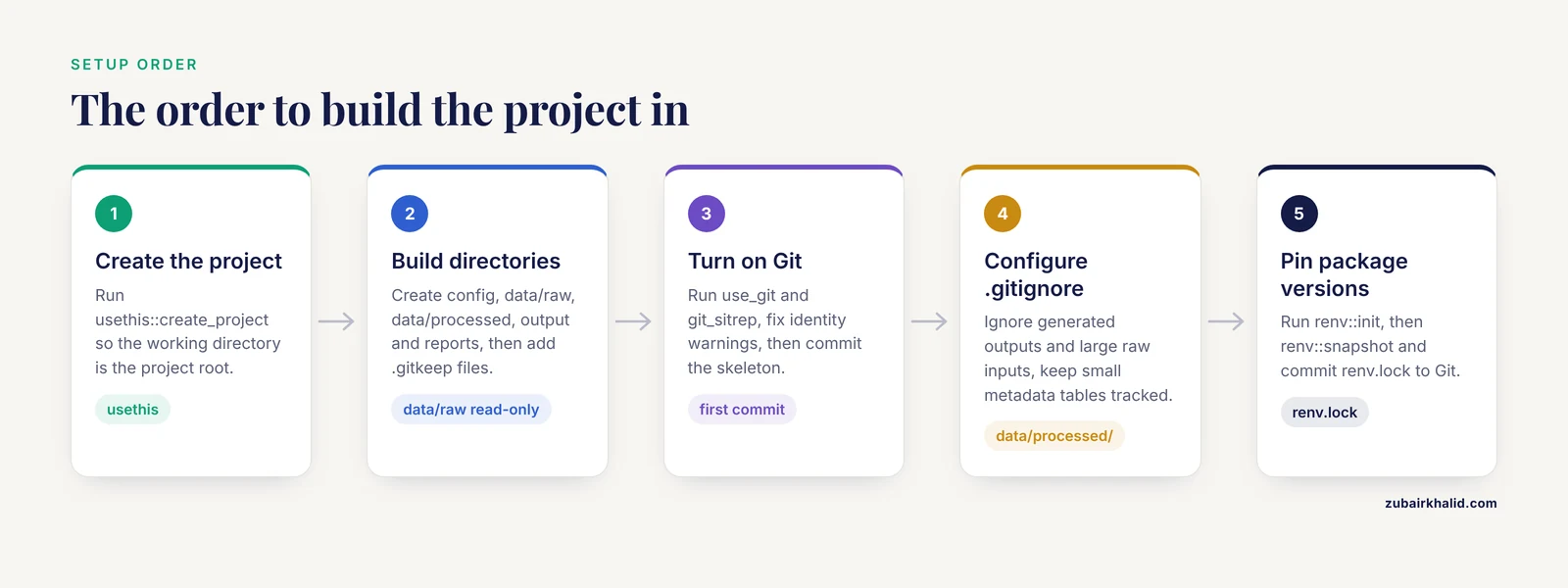
Step 1. Create the project with usethis

Install the three infrastructure packages and create the project. Run this in an R console.

install.packages(c("usethis", "renv", "targets"))
usethis::create_project("~/projects/rnaseq-diet-2026")

Expected output:

✔ Setting active project to '/home/analyst/projects/rnaseq-diet-2026'
✔ Creating 'R/'
✔ Writing 'DESCRIPTION'
✔ Writing 'R/Hello.R'
✔ Modifying '.gitignore'
✔ Opening new project 'rnaseq-diet-2026' in RStudio

RStudio restarts inside the new project. The working directory is now the project root, which matters because every path in your code should be relative to that root. Delete the placeholder R/Hello.R now.

Why usethis::create_project() instead of clicking through RStudio's New Project dialog? The function produces the same result, works identically on Windows, macOS, and Linux, and is scriptable, so you can document your own setup in a bootstrap script.

Step 2. Build the directory skeleton

From the R console inside the project:

dirs <- c(
  "config",
  "data/raw",
  "data/processed",
  "output/figures",
  "output/tables",
  "reports"
)
invisible(lapply(dirs, dir.create, recursive = TRUE))

Empty directories are invisible to Git, so add a placeholder file to each one you want tracked:

file.create(file.path(dirs, ".gitkeep"))

Put your actual raw inputs in data/raw now. For the running example used throughout this walkthrough, that is a gene-level count matrix and a sample metadata table:

# Example only, replace with your real inputs
# data/raw/counts.tsv          genes x samples integer counts
# config/sample_metadata.tsv   sample_id, condition, batch, lib_size

Step 3. Turn on Git before you write code

usethis::use_git()
usethis::git_sitrep()

git_sitrep() reports your configured user name and email and warns if they are missing. Fix any warnings before the first commit, because Git stamps every commit with that identity.

Expected output from use_git():

✔ Adding Git commit of current state
✔ Initializing Git repository

Make the first commit through the RStudio Git pane or the terminal:

git add -A
git commit -m "Project skeleton"

Step 4. Configure .gitignore the bioinformatics way

Open .gitignore and make it contain at least this:

.Rhistory
.RData
.Rproj.user/

# generated outputs are rebuildable, do not track them
data/processed/
output/
*.html

# large raw inputs may be too big for Git, see FAQ
data/raw/*
!data/raw/.gitkeep

The logic: track everything needed to rebuild the analysis, ignore everything the analysis generates. Raw data sits in an awkward middle. Small metadata tables belong in Git. A 40 GB BAM file does not, and the FAQ section covers the standard options for that case. Large consortia face the same question at scale, and the AACR Project GENIE consortium documented how much explicit effort goes into agreeing how data are gathered, harmonized, and shared across institutions, decisions that start with conventions exactly like these [5].

Step 5. Pin your package versions with renv

This is the step that separates a reproducible project from a folder of scripts. renv records the exact version of every package your project uses and can reinstall that exact set later.

renv::init()

Expected output:

- Discovering package dependencies ... Done!
- Copying packages into the project library ... Done!
The following package(s) have been updated:
- renv [1.0.7]
- <your other packages>
* Lockfile written to 'renv.lock'.

Then write real code for a while, and when you add a package with install.packages() or BiocManager::install(), record it:

renv::snapshot()

Expected output:

The following package(s) will be updated in the lockfile:

# CRAN ------------------------------
- cli         [3.6.3]
- usethis     [3.1.0]

# Bioconductor ----------------------
- DESeq2      [1.46.0]

- Lockfile written to 'renv.lock'.

Commit renv.lock to Git. Anyone can now rebuild your environment:

renv::restore()

The lockfile records package name, version, source, and a cryptographic hash of each package, so restore() installs byte-identical versions. This addresses workflow decay directly, because the standardized infrastructure survives even when the original analyst has moved on to a different computer [2].

Step 6. Declare dependencies in DESCRIPTION

Even for an analysis project and not a package, a DESCRIPTION file is the machine-readable list of what your project needs. Open it and reduce it to this form:

Package: rnaseqdiet
Title: Diet effects on mouse liver transcriptome
Version: 0.0.1
Description: Differential expression analysis of the 2026 diet study.
Depends: R (>= 4.3.0)
Imports:
    DESeq2,
    dplyr,
    ggplot2,
    readr,
    targets
Config/PkgType: analysis

The Imports field documents intent, renv.lock documents exact versions, and the two together answer different questions from future readers. Depends: R (>= 4.3.0) sets the minimum R version, which matters because Bioconductor releases are tied to specific R versions, a point covered in the Bioconductor section below.

Step 7. Put logic in R/, parameters in config/

A well-structured project has almost no interactive code in scripts. Instead, each analytical step is a function in R/, and a small config file holds the values you would otherwise hardcode.

Create R/qc_counts.R:

#' Filter low-count genes from a count matrix
#'
#' @param counts Integer count matrix, genes in rows, samples in columns.
#' @param min_count Minimum count required in at least one sample.
#' @return The filtered count matrix.
filter_low_counts <- function(counts, min_count = 10) {
  stopifnot(is.matrix(counts), is.numeric(counts))
  keep <- rowSums(counts) >= min_count
  message(sprintf("Kept %d of %d genes", sum(keep), nrow(counts)))
  counts[keep, , drop = FALSE]
}

Create config/params.R:

project_params <- list(
  counts_file     = "data/raw/counts.tsv",
  metadata_file   = "config/sample_metadata.tsv",
  min_count       = 10,
  contrast        = c("condition", "highfat", "control"),
  fdr_cutoff      = 0.05
)

Now the analysis script contains no magic numbers. Changing the FDR threshold means editing one config line, and the provenance of every threshold is visible in version control. Published pipeline protocols emphasize exactly this kind of harmonized parameterization across stages as a reproducibility mechanism [4].

A naming convention helps as projects grow. The MeTime package for longitudinal metabolomics, an open-source R package built around a central S4 container that stores datasets, metadata, and analysis outputs, organizes its functions by prefix, with data transformations under mod_*, calculations under calc_*, and meta-analyses under meta_*, so the workflow stays transparent and easy to modify [6]. Adopting the same idea in your own R/ folder, for example read_*, qc_*, model_*, plot_*, gives collaborators a predictable map.

Step 8. Wire it together with targets

Standalone scripts run top to bottom, even when nothing upstream changed. The targets package makes the pipeline dependency-aware: each step is a target, and tar_make() rebuilds only the targets whose inputs changed.

Create _targets.R in the project root:

library(targets)
library(tarchetypes)

source("R/qc_counts.R")
source("config/params.R")

list(
  tar_target(counts_file, project_params$counts_file, format = "file"),
  tar_target(meta, read.delim(project_params$metadata_file)),
  tar_target(counts_raw, as.matrix(read.delim(counts_file, row.names = 1))),
  tar_target(counts, filter_low_counts(counts_raw, project_params$min_count)),
  tar_target(dds, DESeq2::DESeqDataSetFromMatrix(
    countData = round(counts),
    colData   = meta,
    design    = ~ batch + condition
  )),
  tar_target(res, DESeq2::results(DESeq2::DESeq(dds),
    contrast = project_params$contrast)),
  tar_target(sig_table, as.data.frame(
    subset(res, padj < project_params$fdr_cutoff)
  )),
  tar_render(reports/de_report.qmd)
)

Run the pipeline:

tar_make()

Expected output:

▶ dispatched target counts_file
▶ dispatched target meta
▶ dispatched target counts_raw
▶ dispatched target counts
● completed target counts [1.2s]
● completed target dds [4.8s]
● completed target res [9.3s]
● completed target sig_table [0.1s]
● completed pipeline [16.7s]

Run tar_make() again immediately and you get this instead:

✔ skipped target counts_file
✔ skipped target meta
✔ skipped target counts_raw
✔ skipped target counts
✔ skipped pipeline [0.2s]

That skip list is the payoff of structure. The pipeline knows nothing changed, so a full rerun takes under a second. Edit one value in config/params.R and only the downstream targets rebuild. The three-stage shape here, inputs, primary computation, downstream statistics and reporting, matches the stage structure used in published best-practice protocols for sequencing analysis, including their explicit quality control checkpoints between stages [4].

Check what the pipeline knows at any time:

tar_visnetwork()   # interactive dependency graph
tar_manifest()     # printed list of every target and its command

Step 9. Write reports humans can read

Quarto documents in reports/ combine prose, code, and results. A minimal reports/de_report.qmd starts like this:

---
title: "Differential expression: high-fat vs control"
params:
  date: 2026-11-11
---

tar_load(sig_table) tar_load(res)

## Volcano plot

#| label: fig-volcano #| fig-width: 6 #| fig-height: 5 plot(-log10(res$padj), res$log2FoldChange)

Render it from the pipeline or by hand:

quarto::quarto_render("reports/de_report.qmd")

The output is a self-contained HTML file that records the code, the package versions from your sessionInfo() block, and the numbers behind every claim. Automatically generated HTML and PDF reports are the reporting mechanism used by reproducible R packages designed for omics workflows, and retaining intermediate results and provenance alongside them is what makes iterative exploration safe [6].

Step 10. Write the README and record the session

usethis::use_readme_md()

Edit README.md to contain at minimum: one sentence on what the project does, the exact commands to reproduce it (renv::restore(), then tar_make()), and a pointer to the report files. Then create R/session_info.R and source it at the end of every report:

report_session_info <- function() {
  cat("R version:", R.version.string, "\n")
  print(sessionInfo())
}

sessionInfo() captures the R version, locale, and attached packages of the run that produced a given report. It is weaker than renv.lock, because it does not capture package hashes, but it belongs in every rendered report as a per-run fingerprint.

Commit everything and push:

git add -A
git commit -m "Pipeline, config, report, lockfile"
git push

The Bioconductor layer

Much of R for bioinformatics runs on Bioconductor, the open-source project for genomic data analysis packages. Three conventions matter for project structure.

First, install and check through BiocManager:

if (!requireNamespace("BiocManager", quietly = TRUE)) {
  install.packages("BiocManager")
}
BiocManager::install(c("DESeq2", "SummarizedExperiment", "GenomicRanges"))
BiocManager::valid()

BiocManager::valid() compares your installed package versions against the versions for your Bioconductor release and reports any that are out of date. renv and BiocManager work together, because renv::snapshot() detects Bioconductor packages and records them under a Bioconductor section in the lockfile with their repository and version.

Second, respect the release-to-R-version binding. Bioconductor publishes two releases per year, and each release requires a minimum R version, so a lockfile built under Bioconductor 3.19 will not restore cleanly under an R version that predates it. Record both in your README.

Third, use the standard container classes instead of ad hoc data frames where you can. A SummarizedExperiment object holds the count matrix together with per-gene and per-sample metadata in one validated object, so the counts and the metadata cannot drift apart. Packages built on this principle show its value at scale. MeTime stores multiple datasets, metadata, and analysis outputs in a single S4 container and retains provenance across every transformation, which is what allows whole workflows to remain transparent and easy to modify [6]. In your own project, the practical version of this rule is simple: never keep a counts matrix in one variable and its sample metadata in an unordered separate one.

If you are following a Bioconductor tutorial, map its steps into this structure rather than running them as loose scripts. The tutorial's loading step becomes a target in _targets.R, its modeling step becomes a function in R/, and its figures become report chunks in reports/.

When R alone is not enough: the workflow engine boundary

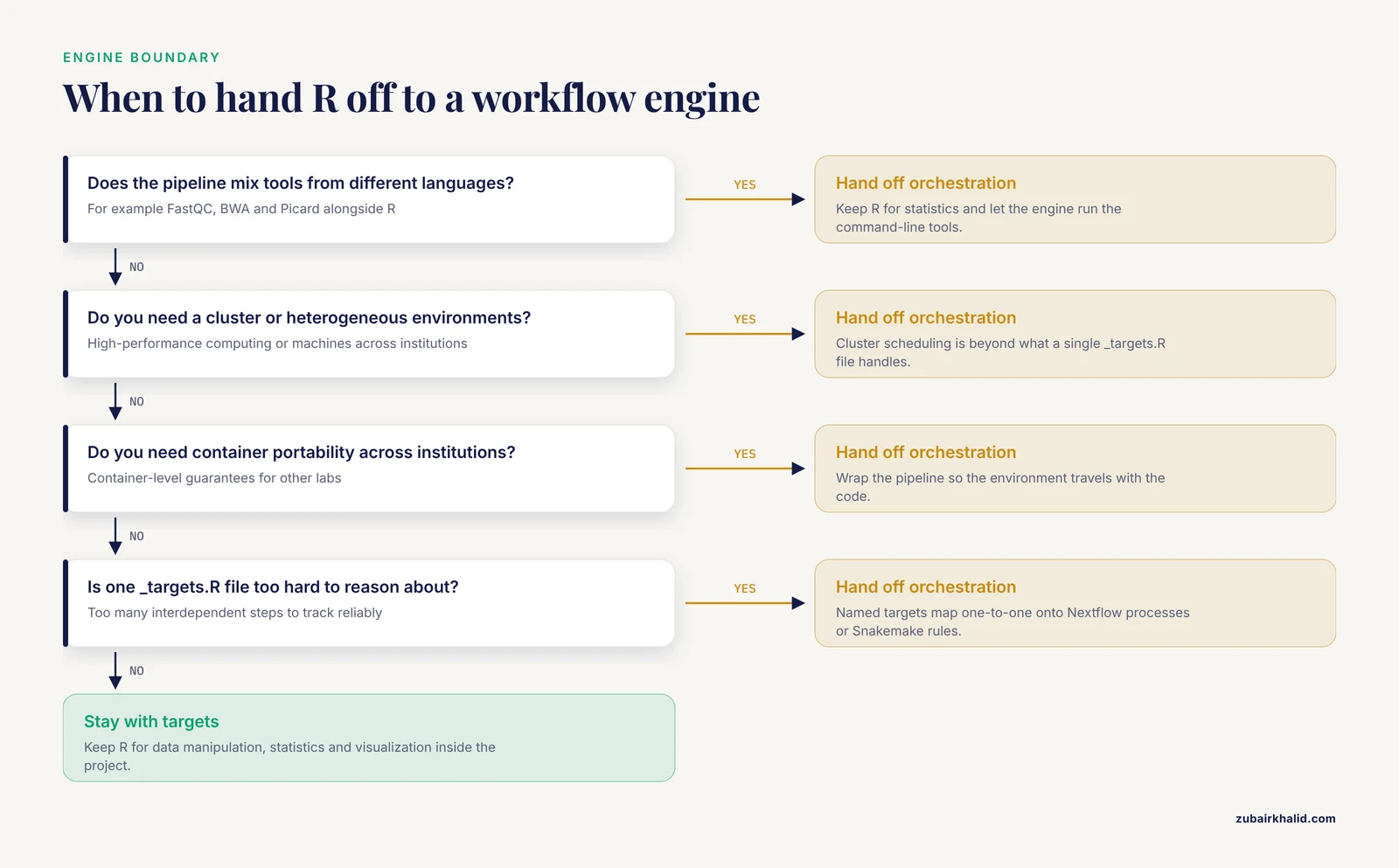
R projects scale beautifully to hundreds of samples. They scale poorly to pipeline logic that involves external command-line tools, cluster scheduling, or multi-language steps. Know the boundary.

A published example shows the pattern clearly. The tcga-data-nf workflow downloads, preprocesses, and analyzes thousands of TCGA samples to infer regulatory networks, with the pipeline logic in Nextflow and the R-specific data management, mapping, and filtering isolated in a standalone companion R package called NetworkDataCompanion [7]. The R package is a clean, testable unit inside a larger workflow. Similarly, the GCAC system for virtual screening model building combines R statistical packages and literate programming tools inside the Galaxy workflow system, using the workflow engine to guarantee reproducibility and automated configuration around R-based steps [8].

The practical rule for your project: keep R for everything that is data manipulation, statistics, and visualization, and hand off orchestration when you hit any of these conditions:

• the pipeline mixes tools from different languages, for example FastQC, BWA, and Picard alongside R [4]
• you need to run on a high-performance computing cluster or across heterogeneous environments [1]
• you need container-level portability guarantees across institutions [1]
• the number of steps makes a single _targets.R file hard to reason about

The good news is that the structure in this article converts cleanly. A targets pipeline already has named, dependency-tracked steps, which map one-to-one onto processes in Nextflow or rules in Snakemake. Your R/ functions become the payload of those processes, your config/ becomes the parameter sheet, and your renv.lock travels inside the container image. Reviews of workflow reuse in bioinformatics found that modularity and clear interfaces are what determine whether a pipeline actually gets reused, which is precisely what this structure produces [3].

Choosing and checking your structure

The table below summarizes the records that make a structured R project verifiable, what each one captures, and what it proves to a future reader.

To check that your structure actually works, run the rebuild test on a clean machine or at minimum a fresh R library:

1. Clone the repository.
2. Run renv::restore() and confirm it completes with no errors.
3. Run tar_make() from scratch after deleting data/processed and output.
4. Confirm the rendered report reproduces the committed figures.

If all four pass, the project is reproducible in the strict sense. H3ABioNet applied an analogous standard across its four production workflows, testing them across heterogeneous computing environments precisely because reproducibility claims mean little until someone else has run them [1].

Common Mistakes and Limitations

• Keeping raw data and analysis code in the same directory level. If data/raw sits inside a folder a collaborator might rsync or Git-track by accident, the first 40 GB commit will hurt. Keep raw inputs outside Git or ignored, as shown in step 4.
• Absolute paths anywhere in the code. read.csv("/Users/alice/data/counts.tsv") runs on exactly one computer. Every path in a structured project is relative to the project root, and the working directory is guaranteed by opening the .Rproj file.
• Using only sessionInfo() for reproducibility. It records attached packages but not versions of packages loaded indirectly or package hashes, so two sessions with identical sessionInfo() output can still behave differently. Use renv.lock as the primary record and sessionInfo() as the per-run addendum.
• Editing files in data/raw. The moment a raw input is touched by hand, its provenance chain breaks and no amount of structure recovers it. If a raw file needs correction, transform it in code into data/processed.
• Treating a notebook as the whole analysis. A Quarto or R Markdown document is a report, not a pipeline. If the notebook is the only artifact, nothing enforces the order of execution or detects stale outputs. Keep the computation in targets and let reports consume pipeline outputs, the division used in the walkthrough above and in published protocol designs that separate computation from explicit downstream reporting [4].
• Ignoring the scalability boundary. A 5,000-line R script handling terabyte-scale inputs and cluster scheduling is the failure mode that pipeline reviews identify when scripting alone is stretched beyond its scale [3]. Plan the workflow-engine handoff before you hit it, not after.
• Hardcoding thresholds in scripts instead of config. When the FDR cutoff lives in five scripts, someone will change it in three of them. The config file plus targets dependency tracking makes the change propagate predictably.
• Skipping Bioconductor version discipline. Installing Bioconductor packages from mixed releases produces subtly wrong results that are nearly impossible to diagnose. Check with BiocManager::valid() and record the release in the README.
• One honest limitation of any structure: it records decisions, it does not make them. Individual analyses still require domain judgment about model design, batch effects, and biological interpretation, and that judgment lives in the prose of your reports rather than in the directory layout.

Frequently Asked Questions

What does a good r project structure bioinformatics example look like?

It separates immutable raw data, generated intermediates, reusable functions, configuration, and human reports into fixed directories, with renv.lock pinning package versions and a _targets.R file defining the pipeline. The full example in this article, built around a differential expression project, shows every directory and file in its expected place.

Is there a standard r project structure bioinformatics format across labs?

No single enforced standard exists, but the layout in this article matches the conventions used by published bioinformatics workflows and R packaging practice, and it converts cleanly into Nextflow, Snakemake, or Galaxy structures, which is what makes it interoperable with larger pipeline efforts [3].

Should I turn my analysis into a proper R package?

For analyses you will rerun, share, or extend, yes. A package gives you namespaces, tests, and documentation for free, and the DESCRIPTION file you already wrote becomes the package manifest. Packages designed this way, such as the companion package in the TCGA regulatory network workflow, survive as reusable units inside larger pipelines [7].

Where do large files like FASTQ and BAM files go in the project?

Keep them in data/raw but exclude them from Git with .gitignore entries, and record their locations, checksums, and download commands in the README. For heavy preprocessing, the pattern used in published workflows is to run alignment and methylation extraction outside R and hand R only the compact downstream inputs [4].

Do I need renv if I already use Docker or Conda?

Use both levels. Conda and Docker pin the system layer, including R itself and external tools, while renv.lock pins the exact R package versions and their hashes inside that system. Consortia running identical analyses on heterogeneous computing environments rely on this combined portability [1].

When should I move my R analysis into Snakemake or Nextflow?

Move when the pipeline mixes command-line tools with R, needs cluster scheduling, or has grown too many interdependent steps to track reliably in a single project. Reviews of pipeline practice identify exactly this scale threshold where workflow systems become necessary for maintainability and reuse [3].

How does this structure relate to a Bioconductor tutorial?

Map each tutorial step into the structure: data loading becomes a target, analysis functions go in R/, and figures go in a Quarto report in reports/. Install tutorial packages with BiocManager, verify versions with BiocManager::valid(), and let renv::snapshot() capture them in the lockfile.

How do I hand the project to a collaborator so they can rerun it?

Push the repository with renv.lock committed, and put three commands in the README: clone, renv::restore(), and tar_make(). If your collaborator uses a different operating system or cluster, wrap the pipeline in a container or a workflow engine so the environment travels with the code, the approach used for cross-institution workflows [1].

Sources

1. Developing reproducible bioinformatics analysis workflows for heterogeneous computing environments to support African genomics.
2. An evolving computational platform for biological mass spectrometry: workflows, statistics and data mining with MASSyPup64.
3. Developing and reusing bioinformatics data analysis pipelines using scientific workflow systems.
4. A Guide to Enzymatic Targeted Methylation Sequencing Bioinformatics Workflow: Best Practices.
5. American Association for Cancer Research Project Genomics Evidence Neoplasia Information Exchange: From Inception to First Data Release and Beyond-Lessons Learned and Member Institutions' Perspectives.
6. MeTime: an R package for reproducible longitudinal metabolomics data analysis.
7. Reproducible processing of TCGA regulatory networks.
8. GCAC: galaxy workflow system for predictive model building for virtual screening.