How to Perform Statistical Analysis in Python for RNA-Seq Data
By Dr. Zubair Khalid, DVM, MS, PhD ·

By the end of this guide you will be able to take a raw gene-by-sample count matrix, clean and normalize it, fit a proper statistical model to it, and produce a ranked table of differentially expressed genes with adjusted p values, all inside Python. You will need a machine with Python 3.9 or later, a terminal, and roughly 4 to 8 GB of RAM for a typical bulk RNA-seq dataset of 20,000 genes and 20 to 50 samples. Everything shown here runs on Linux, macOS, and Windows via WSL.
Statistical analysis is the step where RNA-seq stops being a pile of aligned reads and starts being biology. A differential expression call is a hypothesis test, and the quality of that test depends on choices you make before you ever press enter: which counts you keep, how you normalize, and which model you fit. Several reviews have pointed out that the field still lacks universally accepted standards for normalization and statistical testing, and that methods built to answer the same question can rest on quite different statistical assumptions [1]. That is exactly why you should understand what your Python tools are doing rather than treating them as black boxes.
Why Python for RNA-Seq Statistical Analysis
Python for bioinformatics has historically been strong on data wrangling, machine learning, and visualization, while R held the crown for differential expression through packages like DESeq2 and edgeR. That gap has closed. PyDESeq2 is a Python implementation of the DESeq2 workflow for bulk RNA-seq differential expression, released under the MIT license, and its authors report better precision and speed improvements on large datasets such as TCGA cohorts compared with the original R implementation [2]. The same group has since extended the approach to federated settings, where FedPyDESeq2 runs the DESeq2 pipeline across siloed datasets without moving raw patient data, and achieves near-identical results to pooled analysis on TCGA benchmarks [3].
On the single-cell side, Python tools such as scanpy and scedar handle exploratory analysis of datasets with millions of cells. Scedar, for example, provides scalable visualization, dropout imputation, rare-profile detection, and clustering built on extensible high-performance data structures [4].
The practical takeaway is that you can now run an end-to-end statistical analysis, from count matrix to volcano plot, without leaving Python, and you keep the flexibility of pandas, NumPy, and scikit-learn for everything downstream.
The Statistical Problem in RNA-Seq Counts
RNA-seq gives you counts of reads assigned to each gene in each sample. Counts are non-negative integers with variance tied to the mean, and biological replicates add extra variability beyond what a Poisson model would predict. The workhorse distribution for this data is the negative binomial, which adds a gene-specific dispersion parameter on top of Poisson sampling noise. A statistical review of RNA-seq methods describes how analysis questions arise at the sample, gene, transcript, and exon levels, and compares the assumptions of the models commonly used at each level [1].
Two ideas from the count-modeling literature matter for everything that follows:
- Gene-specific dispersion. Assuming one common dispersion across all genes discards real information. Empirical Bayes methods let each gene have its own variability estimate even with few replicates, and genes whose results are inconsistent across replicates get de-prioritized automatically [5]. This is the core of edgeR's generalized linear model framework and, in modified form, of DESeq2 and PyDESeq2.
- Normalization before testing. Sequencing depth differs between libraries, sometimes by several-fold. Comparing raw counts between samples of different depth inflates false positives for genes simply expressed at higher absolute levels in deeply sequenced samples.
Normalization choice is not cosmetic. In a controlled comparison using the MAQC datasets with small sample replicates, upper-quartile normalization with a pooled geometric mean (UQ-pgQ2) combined with an exact test achieved better power and specificity than upper quartile, TMM, or RLE normalization alternatives [6]. Separately, the PANDORA p value combination approach was shown to produce differential expression lists largely insensitive to the choice of normalization method, suggesting a way to hedge against that choice [7]. You do not need to implement these methods yourself, but you should know they exist and that the default is not the only defensible option.
A Step-by-Step Python RNA-Seq Statistical Analysis Workflow
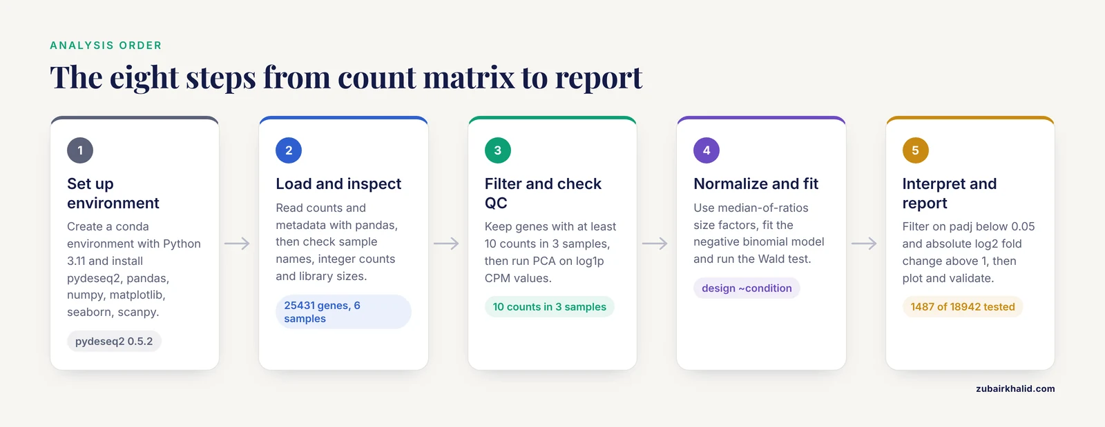
This walkthrough uses PyDESeq2 on a hypothetical bulk RNA-seq experiment: 6 samples, 3 treated and 3 control, with a count matrix of about 25,000 genes. The same code scales to hundreds of samples.
Step 1: Set Up the Environment
Create an isolated environment so package versions stay reproducible.
conda create -n rnaseq python=3.11
conda activate rnaseq
pip install pydeseq2 pandas numpy matplotlib seaborn scanpy
If conda's solver stalls, install a faster solver first:
conda install -n base conda-libmamba-solver
conda config --set solver libmamba
Check the installation:
python -c "import pydeseq2; print(pydeseq2.__version__)"Expected output is a version string such as 0.5.2. Pin this version in a requirements.txt file and commit it to your repository so a collaborator can reproduce your numbers exactly.
Step 2: Load and Inspect the Count Matrix and Metadata
Your two inputs are a count matrix (genes as rows, samples as columns, raw integers) and a sample metadata table (samples as rows, experimental factors as columns). A featureCounts, Salmon, or kallisto output can be reformatted into this shape with pandas.
import pandas as pd

counts = pd.read_csv("counts.csv", index_col=0)
metadata = pd.read_csv("metadata.csv", index_col=0)

print(counts.shape)        # (25431, 6)
print(metadata.condition)  # control or treatment
Before anything else, verify three invariants. The sample order in counts.columns must match the row index of metadata. The counts must be non-negative integers. And no sample should be a wild outlier in total count, which would signal a library preparation failure rather than biology.
# 1. Matching sample names
assert list(counts.columns) == list(metadata.index), "Sample names do not align"

# 2. Integer counts
if not (counts % 1 == 0).all().all():
    raise ValueError("Count matrix contains non-integer values. "
                     "Use raw counts, not TPM or FPKM.")

# 3. Library size sanity check
lib_sizes = counts.sum(axis=0)
print(lib_sizes)
print(lib_sizes / lib_sizes.median())
Expected output for a healthy dataset looks like this:
sample_1    21.4M
sample_2    22.1M
sample_3    20.9M
sample_4    22.8M
sample_5    21.7M
sample_6    21.2M
as ratios near 1.0. A sample at 0.4 or 2.5 deserves investigation before any statistics.
Step 3: Filter Low-Count Genes and Run Quality Control
Genes with almost no reads carry no statistical information and add thousands of pointless tests. A standard, defensible rule is to keep genes with at least 10 counts in a minimum number of samples. PyDESeq2's underlying DESeq2 logic filters automatically, but explicit filtering keeps your object smaller and your PCA interpretable.
import numpy as np

# Keep genes with >= 10 raw counts in at least 3 samples
genes_to_keep = counts.columns.map(
    lambda c: True
)  # placeholder removed below
keep = (counts >= 10).sum(axis=1) >= 3
counts = counts.loc[keep]
print(counts.shape)  # typically drops 30-50% of rows
Then look at sample-level structure with a PCA on variance-stabilized-like values. For a quick pre-normalization check, log1p of CPM works:
import scanpy as sc
import anndata as ad

adata = ad.AnnData(counts.T)   # samples as observations
sc.pp.normalize_total(adata, target_sum=1e6)
sc.pp.log1p(adata)
sc.pp.scale(adata, max_value=10)
sc.tl.pca(adata)
sc.pl.pca(adata, color=None)
What you want to see is treated and control samples separating along the first or second principal component only if you expect a strong treatment effect, and no sample drifting off on its own, which would suggest a batch or quality problem. Clustering and PCA at this stage are the same first-line checks used in published plant and animal RNA-seq workflows, where samples are routinely grouped or split by condition before testing [8].
Step 4: Choose a Normalization Strategy
For a standard two-group comparison, the size-factor normalization built into DESeq2 (the RLE-style median-of-ratios approach) is the sensible default, and PyDESeq2 applies it for you. The evidence base for alternatives is worth knowing:
- Median-of-ratios (RLE) and TMM correct for compositional and depth differences and are the defaults in DESeq2 and edgeR respectively.
- Upper quartile normalization and the newer UQ-pgQ2 variant performed best on power and specificity in one benchmark of balanced two-group comparisons with small replicate numbers [6].
- A p value combination strategy such as PANDORA can make your DE gene list robust to whichever normalization you picked, at the cost of running the analysis more than once [7].
One firm rule: never feed TPM, FPKM, or RPKM values into a count-based statistical model. Those are length- and depth-scaled expression units, not counts, and the negative binomial model requires the raw integer counts to estimate dispersion correctly. The error you get if you forget is silent, not loud, which makes it worse.
Step 5: Fit the Negative Binomial Model with PyDESeq2
Now the core statistical analysis. PyDESeq2 wraps the DESeq2 pipeline: size factor estimation, dispersion estimation with shrinkage toward a fitted trend, and a Wald test per gene.
from pydeseq2.dds import DeseqDataSet
from pydeseq2.ds import DeseqStats

# Build the model object
dds = DeseqDataSet(
    counts=counts,             # genes x samples, raw integers
    metadata=metadata,         # samples x factors
    design="~condition",       # formula: what explains expression
    refit_cooks=True,          # refit outliers flagged by Cooks distance
    n_cpus=4,
)

# Run normalization, dispersion estimation, and model fitting
dds.deseq2()

# Statistical testing: treatment vs control
stat_res = DeseqStats(dds, contrast=("condition", "treatment", "control"))
stat_res.summary()
Expected console output includes lines like:
Fitting size factors...
... done in 0.12 seconds.
Fitting dispersions...
... done in 3.41 seconds.
Fitting MAP dispersions...
... done in 1.87 seconds.
Fitting dispersions trend...
... done in 0.55 seconds.
Log-fold changes calculation & Wald tests...
... done in 5.02 seconds.
Key parameters to understand:
- design: an R-style formula.
"~condition"tests treatment against control. For a paired design use"~patient + condition", which models each patient as a blocking factor. The generalized linear model framework that supports this kind of multi-factor design, while separating biological from technical variation, was established in the edgeR literature and carries over directly to DESeq2-style tools [5]. - refit_cooks: when True, samples flagged as outliers by Cooks distance for a given gene are replaced with fitted values and the gene is refit, which protects against a single bad library driving a spurious call.
- contrast: the tuple
(variable, level_of_interest, reference_level)sets the direction of the log2 fold change.
For small studies, apply fold change shrinkage, which reduces the large fold changes that arise from genes with low counts:
stat_res.lfc_shrink(coord="condition[T.treatment]")
res = stat_res.results_df
print(res.head())
Expected output:
              baseMean  log2FoldChange     lfcSE      stat    pvalue      padj
gene_101        812.4           2.31      0.21     10.98  4.7e-28  8.3e-24
gene_207         45.9           1.87      0.35      5.34  9.2e-08  3.1e-05
gene_542      12033.6          -1.12      0.09    -12.44  1.6e-35  5.9e-30
Step 6: Interpret the Results Table
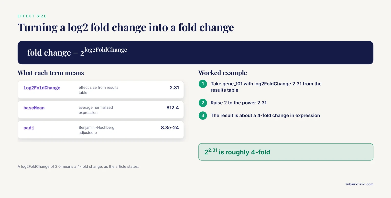
Each column answers a different question:
- baseMean: average normalized expression. Genes with tiny baseMean have unstable fold changes even at significant p values.
- log2FoldChange: effect size. A value of 2.0 means a 4-fold change in expression.
- pvalue: the Wald test result for that gene, testing whether the fold change differs from zero.
- padj: the Benjamini-Hochberg adjusted p value, which controls the false discovery rate across the thousands of simultaneous tests. This is the column you filter on.
A common reporting standard is padj < 0.05 combined with an effect size threshold:
sig = res[(res.padj < 0.05) & (res.log2FoldChange.abs() > 1)]
print(f"{len(sig)} significant genes out of {len(res)} tested")
Expected output: something like 1487 significant genes out of 18942 tested.
Report the number tested, the thresholds, and the number of hits. Those three numbers let a reviewer reconstruct your result.
Step 7: Visualize the Results
Three plots carry most of the diagnostic value.
import matplotlib.pyplot as plt
import seaborn as sns

# Volcano plot
res["-log10_padj"] = -np.log10(res.padj.fillna(1))
sns.scatterplot(
    data=res, x="log2FoldChange", y="-log10_padj",
    hue=(res.padj < 0.05) & (res.log2FoldChange.abs() > 1),
    s=8, legend=False,
)
plt.axhline(-np.log10(0.05), ls=":", c="grey")
plt.axvline(1, ls=":", c="grey")
plt.axvline(-1, ls=":", c="grey")
plt.savefig("volcano.png", dpi=300)

# MA plot: fold change vs mean expression
stat_res.plot_MA()
plt.savefig("ma_plot.png", dpi=300)

# Heatmap of top genes across samples
top = res.sort_values("padj").head(30).index
sns.clustermap(np.log1p(counts.loc[top]), cmap="viridis")
plt.savefig("heatmap.png", dpi=300)
Read the MA plot first. A healthy analysis shows a funnel: fold change estimates shrink toward zero as mean expression decreases. If low-count genes show enormous fold changes with no shrinkage, your model fitting went wrong or you skipped shrinkage.
Step 8: Validate and Report
Three checks separate a trustworthy result from a lucky one. First, confirm that your positive control genes, if you have any known treatment-responsive markers, appear among the hits. Second, check the direction of the fold changes for genes in the pathway you expect the treatment to affect. Third, compare your hit count against the size of your study. Method comparison studies have shown that with only 3 replicates per group, method choice materially affects false discovery rate control and power, while with 6 or more replicates the major methods converge in performance [9]. If you ran a 3-versus-3 experiment and found 8,000 significant genes, treat the result as a hypothesis list, not a conclusion.
Choosing Between Statistical Methods in Python
The table below summarizes your realistic options and how to reach each from Python.
| Method | Statistical model and test | Best suited for | Python access |
|---|---|---|---|
| PyDESeq2 | Negative binomial GLM, Wald test, optional LFC shrinkage | Bulk RNA-seq, two-group and multi-factor designs, medium to large n | Native package [2] |
| edgeR logic | Negative binomial GLM, exact test or quasi-likelihood F test | Balanced two-group comparisons, small replicates | Via rpy2 calling R, or PyDESeq2 as the closest native equivalent [6] |
| PANDORA-style p value combination | Combines p values across normalization pipelines | Hedging against normalization choice, transcript types such as long non-coding RNAs | Implement the combination step in pandas/NumPy [7] |
| Voom-style linear modeling | Log-count precision weights, linear model | Complex designs, factorial experiments | Via rpy2, or limma-voom wrappers |
| Non-parametric tests | Mann-Whitney U and related rank tests | Platform comparison studies, small n without distributional assumptions | scipy.stats.mannwhitneyu [10] |
No single method wins everywhere. A large simulation study comparing edgeR, DESeq, DESeq2, baySeq, EBSeq, NOISeq, SAMSeq, and voom found no significant differences in false discovery rate control, power, or stability across methods for equal or unequal library sizes, with EBSeq performing best at 3 replicates per group and DESeq2 performing best at 6 or 12 replicates per group under negative binomial count data [9]. In practice, PyDESeq2 gives you the best-documented Python-native path, and simulation studies confirm DESeq2-style workflows hold up at moderate replicate numbers [9].
Python RNA-Seq Statistical Analysis Tips
These tips address the decisions that most often change your results.
Tip 1: Design your formula before you look at results. The design formula determines which variation the model explains away. If you have batch, sex, or patient identity, put it in the formula as a blocking term. The multi-factor GLM framework exists precisely so that treatment effects can be estimated while accounting for biological variation between samples [5]. Adding a factor after seeing your results is a form of p hacking.
Tip 2: Prefer biological replicates over sequencing depth. Depth helps you detect genes, replicates give you the degrees of freedom to call anything significant. Method evaluations consistently show replicate number, not read depth, driving power differences [9].
Tip 3: Test sensitivity to normalization. Rerun the analysis with a second normalization and compare hit lists. If your top biology survives both, it is robust. If it appears under only one normalization, either investigate the discrepancy or use a combination approach that is explicitly normalization-insusceptible [7].
Tip 4: Shrink fold changes for ranking, use unshrunken values for effect claims. Shrunken log2 fold changes are more stable for ranking and visualization, but if you plan to validate a 2-fold change by qPCR, confirm the number against the unshrunken estimate for genes with adequate count depth.
Tip 5: Save the fitted object. Pickle or save the fitted dds with dds.write("dds.h5ad") if using AnnData-backed PyDESeq2. Refitting takes minutes on large cohorts, and downstream contrast testing becomes a fast re-run rather than a full refit.
Tip 6: Use the Wald test by default, and know what alternatives exist. The Wald test versus the exact test or quasi-likelihood F test is a real methodological fork. One benchmark found UQ-pgQ2 normalization combined with an exact test outperformed other normalization-test pairings for power and specificity in balanced two-group comparisons [6]. PyDESeq2 exposes the Wald test natively, so exact-test comparisons require calling R through rpy2.
Extending the Workflow to Single-Cell RNA-Seq
Single-cell data breaks most bulk assumptions and needs its own statistical treatment. Differential expression analysis of scRNA-seq data has been organized into six major classes of statistical approaches: generalized linear, generalized additive, hurdle, mixture models, two-class parametric, and non-parametric, each addressing limitations of the previous class [11]. Dropout events, where a gene reads as zero in a cell that actually expressed it, are the defining challenge, and methods that model the molecular capture process underlying dropouts have shown improved performance across multiple datasets and protocols [12].
For Python-native single-cell work:
- Use scanpy for standard clustering and marker analysis, and scedar when dataset size demands scalable structures for visualization, imputation, and rare-profile detection [4].
- For normalization of noisy single-cell data before testing, methods designed to remove technical noise while preserving biological variation, such as Linnorm, improved false positive control and accuracy compared with applying bulk methods like DESeq2 directly [13].
- If your question is how a pseudotemporal process differs between conditions and you have multiple samples, use a framework that accounts for cross-sample variability. Lamian is a statistically rigorous framework for differential multi-sample pseudotime analysis that detects changes in gene expression, cell density, and trajectory topology while adjusting for batch effects, and it reduces sample-specific false discoveries that would not generalize to new samples [14].
A caution specific to cancer single-cell work applies broadly: inadequate use of computational methods can produce dubious results, and common pitfalls include statistical errors in differential analysis, overinterpreted trajectory inference, and signature-based analyses applied out of context [15]. The safe rule is to match the statistical method to the actual data structure, not to the most convenient default.
Where Biopython Fits in the Pipeline
If you came here through a Biopython tutorial, know where Biopython belongs and where it does not. Biopython excels at sequence-level tasks: parsing FASTA and GenBank files, working with annotations, translating sequences, and interfacing with NCBI Entrez. It does not provide count-based differential expression statistics. A realistic division of labor is Biopython for fetching gene annotations and reference sequences, a quantification tool such as featureCounts, Salmon, or kallisto for producing the count matrix, and PyDESeq2 for the statistical analysis described above. Keeping these layers separate also keeps your workflow debuggable, because a failure in annotation retrieval looks nothing like a failure in dispersion fitting.
Common Mistakes and Limitations
These are the mistakes that appear repeatedly in real analyses, including in reviews of published single-cell and bulk work [15].
Feeding TPM or FPKM into a count model. The negative binomial model requires raw counts. Normalized expression units destroy the mean-variance relationship the model depends on. Always start from the raw count matrix and let the tool handle normalization internally.
Treating samples as independent when they are not. Three technical replicates of one culture are not three biological replicates. If multiple libraries come from one donor or one animal, they belong to the same biological unit and need a blocking term or mixed model treatment, or your effective sample size is inflated and your p values are optimistic.
Filtering genes on adjusted p values in the control group first. Selecting genes by significance in a separate screen and then testing the same genes in your comparison creates selection bias. Filter on count-based criteria applied uniformly to all samples.
Interpreting an unadjusted p value. With 20,000 genes tested, 0.05 alpha gives you roughly 1,000 false positives by chance alone. The Benjamini-Hochberg adjusted value is the one that controls the proportion of false discoveries among your calls. Adjusted values are frequently reported with validation in scRNA-seq differential expression practice, and skipping them is among the most cited statistical errors in published analyses [11].
Ignoring sample-level outliers. Cooks distance refitting catches gene-level outliers, but a whole-sample quality failure needs to be caught at the PCA and library size stage, before modeling. A sample driven by a different cell type composition will otherwise scatter your results unpredictably.
Overinterpreting small-n results. With 3 versus 3 replicates, the choice of statistical method changes results noticeably, and EBSeq showed the strongest false discovery control in simulations at that sample size [9]. Label such analyses as exploratory and plan validation.
Expecting one normalization to be universally correct. Reviews of normalization and testing combinations report real performance differences between methods, including better power and specificity for specific pairing of normalization with the exact test, and no consensus standard exists [6] [1]. Sensitivity analysis across normalizations is cheap and honest.
Mixing up statistical significance with biological importance. A 0.1 log2 fold change can reach significance in a deeply powered cohort and be irrelevant at the protein level. Report effect sizes alongside adjusted p values, and confirm key genes with an orthogonal assay where the claim matters.
Frequently Asked Questions
Can I run a complete RNA-seq differential expression analysis in Python without using R?
Yes. PyDESeq2 implements the full DESeq2 workflow, from size factor estimation through dispersion fitting to Wald testing and results tables, as a native Python package [2]. For methods with no Python equivalent, such as edgeR's quasi-likelihood test, you can bridge to R through rpy2.
Which statistical test should I use for my two-group RNA-seq comparison?
Use the Wald test with PyDESeq2 as your default, and be aware that benchmarks of normalization and test combinations have found specific pairings, such as upper-quartile-based normalization with an exact test, can improve power and specificity in balanced two-group designs [6]. With 6 or more replicates per group, major methods converge in performance [9].
How many biological replicates do I need?
Plan for at least 3 per group, and prefer 6 or more when the experiment matters. Simulation evidence shows method performance differences are most pronounced at 3 replicates per group, while at 6 and 12 replicates per group DESeq2-style methods performed best on false discovery control, power, and stability [9].
What cutoffs should I use for calling differentially expressed genes?
Use an adjusted p value threshold, typically 0.05 under Benjamini-Hochberg control, and add a log2 fold change threshold as a biological relevance filter. Report both cutoffs and the total number of genes tested so others can reproduce your call set.
Can I use PyDESeq2 on single-cell RNA-seq data?
Not directly as a substitute for single-cell methods. Bulk count models treat one sample as the unit of observation, while scRNA-seq analysis must handle dropout, cell-level overdispersion, and cross-sample variability. Dedicated approaches exist across six statistical model classes for single-cell differential expression [11], and pseudotime comparisons require frameworks that account for sample-level replication [14].
Why does my count matrix need integer values?
The negative binomial model is defined over counts. If you feed TPM, FPKM, or averaged replicates, dispersion estimation is invalid and your p values lose their meaning. Start from raw counts from the quantification step and apply normalization inside the statistical tool.
How do I handle batch effects in Python?
Include batch as a term in your design formula, for example design="~batch + condition", so the model separates known technical variation from the treatment effect. This multi-factor approach, which estimates biological variation separately from other sources, is standard in count-based GLM frameworks [5]. Verify batch correction visually with PCA before and after.
Should I use TPM, FPKM, or raw counts for differential expression?
Raw counts, always, as the input to the statistical model. TPM and FPKM are useful for comparing relative expression within a sample or for visualization, but they are not valid inputs for count-based differential testing, and using them is one of the most common and damaging mistakes in the field [1].
Sources
- Modeling and analysis of RNA-seq data: a review from a statistical perspective
- PyDESeq2: a python package for bulk RNA-seq differential expression analysis
- FedPyDESeq2: a federated framework for bulk RNA-seq differential expression analysis
- Scedar: A scalable Python package for single-cell RNA-seq exploratory data analysis
- Differential expression analysis of multifactor RNA-Seq experiments with respect to biological variation
- Choice of library size normalization and statistical methods for differential gene expression analysis in balanced two-group comparisons for RNA-seq studies
- Integrative, normalization-insusceptible statistical analysis of RNA-Seq data, with improved differential expression and unbiased downstream functional analysis
- Identifying Candidate Genes Related to Soybean (Glycine max) Seed Coat Color via RNA-Seq and Coexpression Network Analysis
- An evaluation of RNA-seq differential analysis methods
- The Role of Microarray in Modern Sequencing: Statistical Approach Matters in a Comparison Between Microarray and RNA-Seq
- Differential Expression Analysis of Single-Cell RNA-Seq Data: Current Statistical Approaches and Outstanding Challenges
- SwarnSeq: An Improved Statistical Approach for Differential Expression Analysis of Single-Cell RNA-Seq Data
- Linnorm: improved statistical analysis for single cell RNA-seq expression data
- A statistical framework for differential pseudotime analysis with multiple single-cell RNA-seq samples
- Pitfalls in analysis and interpretation of single-cell RNA-seq data in cancer