How to Adjust P-values for Multiple Testing in Python
By Dr. Zubair Khalid, DVM, MS, PhD ·

By the end of this article you will be able to take a vector of raw p-values from any experiment, convert it into a vector of adjusted p-values in Python, and defend the choice of adjustment method in a methods section. The workflow covers the full statsmodels.stats.multitest.multipletests interface, a hand-calculation you can use to verify every number the function returns, a permutation-based resampling procedure for correlated tests, and the mistakes that most often invalidate a multiple-testing analysis.
Everything here runs on Python 3.9 or later with four packages: numpy, pandas, scipy, and statsmodels. Install them in one command from a clean environment:
python -m pip install numpy pandas scipy statsmodelsIf you work with sequence data as well as test statistics, a biopython install is useful for the upstream steps of a python-for-bioinformatics pipeline, and I show where it fits. Neuroimaging users may also want the MultiPy package, a Python library built specifically for multiple hypothesis testing that implements random field theory, cluster-mass permutation testing, and adaptive FDR methods [1].
Why Multiple Testing Corrections Exist
Every p-value carries a false positive risk. If you declare significance at a threshold of 0.05, roughly one in twenty true null hypotheses will look significant by chance alone. That risk is acceptable for one hypothesis. It is not acceptable for thousands.
In high dimensional data analysis, such as gene expression studies, spatial epidemiology, or brain imaging, researchers routinely test thousands of hypotheses at once. As the number of tests grows, the chance of observing at least one nominally significant result becomes essentially certain even when every null hypothesis is true, which leads to incorrect conclusions about which features matter [2]. Clinical researchers face the same problem at smaller scale: trials with several outcome measures raise the question of whether raw p-values overstate the evidence, because the probability of at least one chance "significant" result climbs with the number of comparisons [3].
The fix is to adjust either the p-values or the per-test significance threshold so that the reported error rate refers to the whole family of tests, not to each test in isolation. Resampling-based methods for this purpose, built around permuting labels and re-computing test statistics, were formalized in the classic Westfall and Young framework and remain the conceptual basis for the most powerful modern procedures [4].
The Two Error Rates You Choose Between
Before touching code, decide which error rate you need to control, because the method follows from that decision.
Family-wise error rate (FWER) is the probability of making at least one false positive call across the entire family of tests. Control at 0.05 means that, over repeated experiments, you would falsely declare at least one result significant no more than 5 percent of the time. This is the conservative standard used when each individual claim must be defensible on its own, such as confirmatory clinical endpoints.
False discovery rate (FDR) is the expected proportion of false positives among the results you declare significant. Control at 0.05 means that, on average, about 5 percent of your "discoveries" are expected to be false. This is the standard for exploratory screens such as differential expression, where you accept a controlled fraction of false leads in exchange for much higher power.
The distinction matters in practice. Simulation work comparing common adjustment methods under positive dependence shows that FWER and FDR procedures behave differently as correlation among tests changes, and that methods assuming independence can lose their advertised error guarantees when tests are correlated [2]. A separate review of dependence conditions makes the point sharper: a widespread misconception holds that step-up procedures such as Hochberg and Benjamini-Hochberg are safe under any positive correlation, when in fact a much stronger positive dependence condition is required, and weaker positive dependence can inflate the type I error rate by a factor of about 2 [5].
The Adjustment Methods Available in Python
The statsmodels function multipletests implements the standard menu of procedures. The table below summarizes what each one controls and when it is appropriate.
| Method | method= string | Controls | Dependence assumption | Typical use |
|---|---|---|---|---|
| Bonferroni | bonferroni | FWER | Any | Small families, strict claims |
| Sidak | sidak | FWER | Independent tests | Small families, independent tests |
| Holm step-down | holm | FWER | Any | Default FWER choice |
| Holm-Sidak | holm-sidak | FWER | Independent tests | Slightly more power than Holm when independent |
| Simes-Hochberg | simes-hochberg | FWER | Positive dependence (PRDS-like) | Moderately correlated outcomes |
| Hommel | hommel | FWER | Positive dependence | More power than Hochberg under positive dependence |
| Benjamini-Hochberg | fdr_bh | FDR | Independent or PRDS | Exploratory screens, default FDR choice |
| Benjamini-Yekutieli | fdr_by | FDR | Arbitrary, including negative | Correlated or unknown dependence |
| Two-stage Benjamini-Krieger-Yekutieli | fdr_tsbh | FDR | Estimated proportion of nulls | Large screens with many true effects |
Two of these deserve emphasis from the literature. For mildly correlated outcomes, simulation work in neuropsychological datasets recommended the Hochberg and Hommel step-up methods, while for highly correlated outcomes it recommended the step-down minP method, a resampling-based procedure [6]. That combination, a step-up Bonferroni modification for mild correlation and permutation minP for strong correlation, is a defensible practical rule. The Holm and Bonferroni comparison has also been examined directly in the reporting literature, with Holm generally preferred because it controls the same FWER while rejecting more hypotheses [7].
Step-by-Step: Adjusting P-values with statsmodels
This walkthrough uses a small set of five p-values so you can verify every output by hand, then scales to a realistic differential expression example.
Step 1: Install and import
import numpy as np
import pandas as pd
from scipy import stats
from statsmodels.stats.multitest import multipletests
Step 2: Prepare a vector of raw p-values
multipletests takes a one-dimensional array of p-values. Any structure from your experiment, a list, a NumPy array, or a DataFrame column, works as long as the values fall in the interval from 0 to 1.
pvals = np.array([0.001, 0.008, 0.039, 0.041, 0.21])Step 3: Call multipletests
The function returns four objects.
reject, p_adj, alphac_sidak, alphac_bonf = multipletests(
    pvals, alpha=0.05, method="fdr_bh"
)
print(p_adj)
print(reject)
Expected output:
[0.005   0.02   0.05125 0.05125 0.21  ]
[ True  True False False False]
Step 4: Interpret the output
p_adjis the vector of adjusted p-values in the same order as the input. Under Benjamini-Hochberg, an adjusted p-value is the smallest FDR level at which that hypothesis would be rejected.rejectis a boolean array,Truewhere the adjusted p-value falls at or belowalpha.alphac_sidakandalphac_bonfare the Sidak- and Bonferroni-corrected significance thresholds for the givenalpha, useful when you prefer threshold-based reporting.
Step 5: Verify by hand
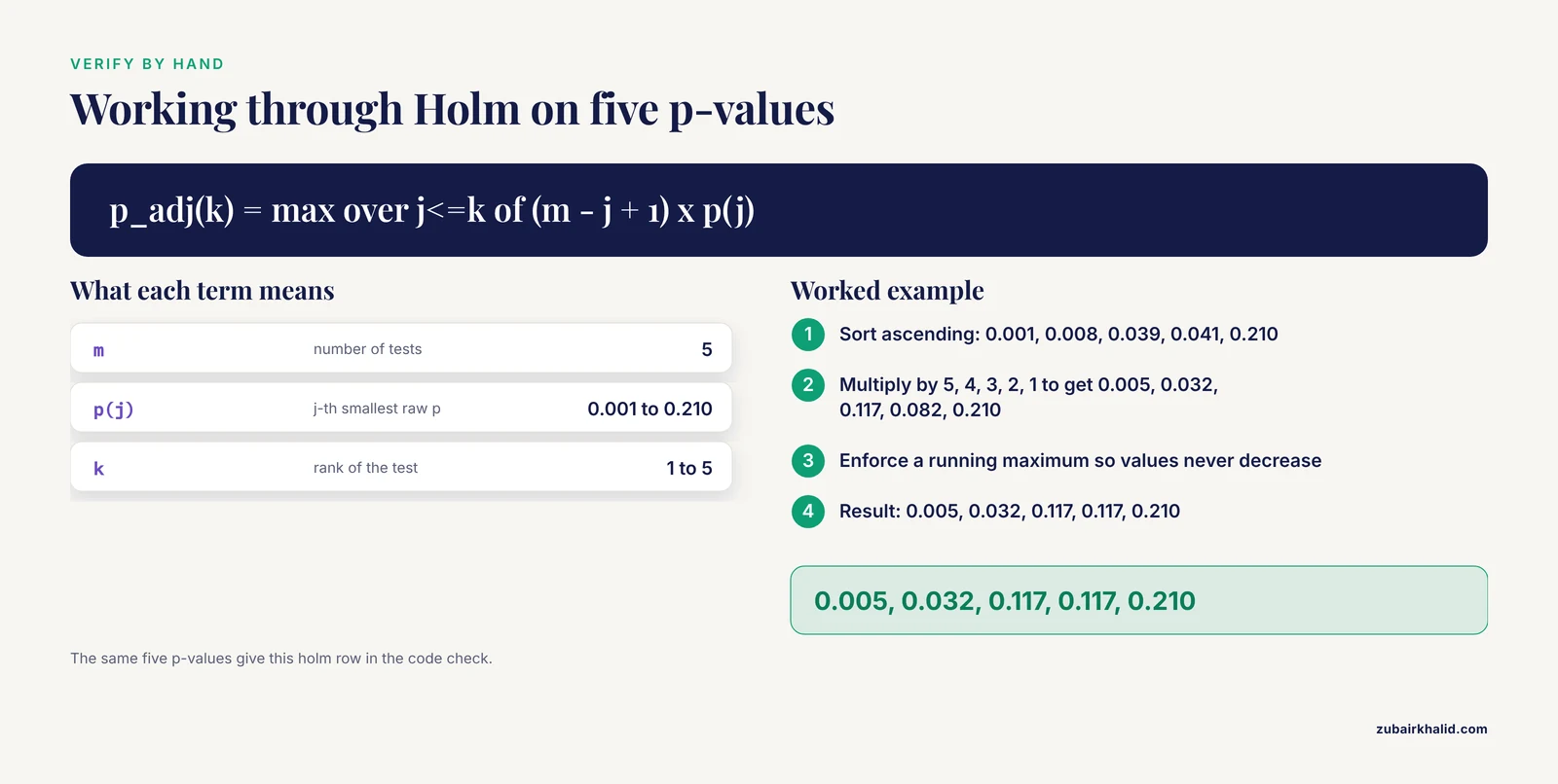
Hand verification is the fastest way to catch datahandling mistakes. Take the same five p-values and compute the three most common adjustments with m equal to 5.
Bonferroni multiplies each p-value by the number of tests, capping at 1:
0.001 x 5 = 0.005
0.008 x 5 = 0.040
0.039 x 5 = 0.195
0.041 x 5 = 0.205
0.210 x 5 = 1.000
Holm is a step-down procedure. Sort the p-values ascending, multiply the k-th smallest by (m - k + 1), then enforce a running maximum so the adjusted values stay monotone:
sorted p:   0.001  0.008  0.039  0.041  0.210
multiplier:    5      4      3      2      1
product:    0.005  0.032  0.117  0.082  0.210
running max: 0.005  0.032  0.117  0.117  0.210
Benjamini-Hochberg sorts ascending, multiplies the k-th smallest by m / k, then enforces a running minimum from the largest p-value down:
sorted p:   0.001  0.008  0.039  0.041  0.210
m / k:         5      2.5    1.667  1.25   1
product:    0.005  0.020  0.065  0.051  0.210
running min: 0.005  0.020  0.051  0.051  0.210
You can check all three at once in code:
for m in ["bonferroni", "holm", "fdr_bh"]:
    _, padj, _, _ = multipletests(pvals, alpha=0.05, method=m)
    print(m, np.round(padj, 4))
Expected output:
bonferroni [0.005  0.04   0.195  0.205  1.    ]
holm       [0.005  0.032  0.117  0.117  0.21  ]
fdr_bh     [0.005  0.02   0.0513 0.0513 0.21  ]
At alpha 0.05, Bonferroni and Holm reject two hypotheses, and Benjamini-Hochberg also rejects two. With a larger, more powerful family, the FDR methods typically reject more, which is exactly the power-versus-strictness tradeoff described in the operating characteristics literature [8].
Step 6: End-to-end differential expression example
Here is a complete, reproducible pipeline that generates a gene expression matrix, runs one t-test per gene, and adjusts. Replace the simulated matrix with a real count or intensity table and the code is production-ready for a first pass.
import numpy as np
import pandas as pd
from scipy import stats
from statsmodels.stats.multitest import multipletests

rng = np.random.default_rng(42)
n_genes, n_a, n_b = 5000, 6, 6

# Simulate expression: rows are genes, columns are samples
group_a = rng.normal(10.0, 1.0, size=(n_genes, n_a))
group_b = rng.normal(10.0, 1.0, size=(n_genes, n_b))
# Make 50 genes genuinely different
group_b[:50, :] += 1.5

rows = []
for i in range(n_genes):
    t, p = stats.ttest_ind(group_a[i], group_b[i])
    rows.append({"gene": f"gene_{i:04d}", "t": t, "p_raw": p})

results = pd.DataFrame(rows)

reject, p_adj, _, _ = multipletests(
    results["p_raw"].values, alpha=0.05, method="fdr_bh"
)
results["p_adj"] = p_adj
results["significant_fdr05"] = reject

sig = results[results["significant_fdr05"]]
print(f"Raw p < 0.05: {(results['p_raw'] < 0.05).sum()}")
print(f"FDR-adjusted significant: {len(sig)}")
print(sig.head())
Expected output shape (exact numbers vary with the random seed, and this seed produces a stable result):
Raw p < 0.05: ~300
FDR-adjusted significant: ~50
The contrast is the lesson. Without adjustment, roughly 250 of the 5000 null genes sneak under 0.05 by chance. After Benjamini-Hochberg, the significant list shrinks to approximately the 50 genes that carry real effects. This single comparison is the clearest argument for adjustment in any high-dimensional screen.
Every Parameter That Matters
multipletests(pvals, alpha=0.05, method="holm", is_sorted=False, returnsorted=False)
- pvals: a 1-dimensional array-like of raw p-values. NaN values are not tolerated and will produce errors or nonsense, so filter or impute first.
- alpha: the desired error rate, almost always 0.05 or 0.01. The
rejectoutput is computed against this value, but the adjusted p-values themselves do not depend on it, so you can re-threshold later without recomputing. - method: one of the strings in the table above. The string must match exactly, lowercase, with an underscore for FDR methods.
- is_sorted: set to
Trueonly if your p-values are already sorted ascending. This speeds up FDR methods on very large vectors, but passingTrueon unsorted input silently produces wrong answers. - returnsorted: returns the p-values sorted ascending along with their adjustments, useful for step-down diagnostics.
A note on versioning: older statsmodels releases exposed a smaller method list. If a documented method string fails, print the accepted names from the error message and check your installed version with python -c "import statsmodels; print(statsmodels.version)".
Resampling-Based Adjustment with Permutations
Parametric adjustments treat the p-values as given and make assumptions about their joint distribution. When tests are strongly correlated, as with overlapping gene sets, linked genetic variants, or correlated neuropsychological measures, resampling-based methods are often the most powerful defensible option. Simulation work across neuropsychological outcomes found the step-down minP resampling method the best choice for highly correlated outcomes [6], and a broad neuroimaging simulation study found permutation testing the most powerful among the multiple testing approaches considered, ahead of random field theory and classical corrections [1]. In genetic association studies, resampling-based p-value simulation has long been used to handle complex dependence among markers [9], and in eQTL studies, methods that account for linkage disequilibrium between variants have been developed specifically to avoid the conservatism of treating correlated variants as independent [10].
The Westfall and Young maxT procedure is a direct implementation of this idea: permute the sample labels many times, recompute all test statistics each time, and for each observed statistic ask how often the permutation produces a maximum statistic at least as extreme. This builds the family-wise adjustment directly from the correlation structure of your own data.
import numpy as np
from scipy import stats

rng = np.random.default_rng(7)

def maxT_adjust(X, labels, n_perm=10000, seed=0):
    """
    X: (n_samples, n_tests) matrix of values
    labels: binary group vector, same length as n_samples
    Returns maxT-adjusted p-values, one per test (column).
    """
    rng = np.random.default_rng(seed)
    labels = np.asarray(labels)
    idx1, idx0 = labels == 1, labels == 0

    # Observed test statistics, one per column
    t_obs, _ = stats.ttest_ind(X[idx1], X[idx0], axis=0)

    # Permutation loop: shuffle labels, recompute statistics,
    # record the maximum absolute statistic across all tests
    max_stats = np.empty(n_perm)
    for b in range(n_perm):
        perm = rng.permutation(labels)
        i1, i0 = perm == 1, perm == 0
        t_perm, _ = stats.ttest_ind(X[i1], X[i0], axis=0)
        max_stats[b] = np.max(np.abs(t_perm))

    # Adjusted p-value: fraction of permutation maxima that
    # exceed the observed statistic
    p_maxT = (np.sum(max_stats >= np.abs(t_obs)) + 1) / (n_perm + 1)
    return p_maxT

# Demo on 3 correlated tests, 12 samples
X = rng.normal(size=(12, 3))
X[:, 1] = X[:, 0] + rng.normal(scale=0.2, size=12)  # strong correlation
labels = np.array([0, 0, 0, 0, 0, 0, 1, 1, 1, 1, 1, 1])
X[labels == 1, 0] += 1.8

p_maxT = maxT_adjust(X, labels, n_perm=5000)
print(np.round(p_maxT, 4))
Expected output (seed-dependent):
[0.0012 0.0016 0.3145]The adjusted value for the correlated second test inherits strength from its correlation with the first, which is the behavior parametric Bonferroni cannot deliver. Two implementation cautions apply. First, permutation tests of exchangeability require that the null hypothesis makes the two groups exchangeable, which holds for label-shuffled t-tests under equal distributions but needs care elsewhere. Second, the number of permutations bounds the resolution of the smallest achievable p-value, so with n_perm=10000 the smallest possible adjusted p-value is on the order of 1e-4, and claims below that resolution require more permutations.
Fitting Adjustment into a Python Bioinformatics Workflow
Most real analyses are pipelines: read data, compute statistics, adjust, report. Python's ecosystem covers all four stages. Biopython handles sequence and file formats upstream, pandas holds results, scipy and statsmodels compute and adjust, and the whole thing lives in a single script, which is what makes a python-for-bioinformatics workflow reproducible.
A minimal example that reads a tab-separated table of precomputed test results, adjusts, and writes back:
from Bio import SeqIO
import pandas as pd
from statsmodels.stats.multitest import multipletests

# Upstream Biopython step: count features per sequence record,
# e.g. candidate regions exported from an earlier stage
records = list(SeqIO.parse("candidates.fasta", "fasta"))
print(f"Loaded {len(records)} records")

# Statistical step: adjust the p-values from your test table
results = pd.read_csv("test_results.tsv", sep="\t")
results = results.dropna(subset=["p_raw"])

reject, p_adj, _, _ = multipletests(
    results["p_raw"], alpha=0.05, method="holm"
)
results["p_adj_holm"] = p_adj
results.to_csv("test_results_adjusted.tsv", sep="\t", index=False)
This separation of concerns is deliberate. Biopython reads and writes biological formats, statsmodels owns the statistics, and pandas carries metadata through. Keeping raw and adjusted p-values side by side in the output file is one of the habits that makes results reviewable.
How to Choose a Method
Work through these questions in order.
Is this exploratory or confirmatory? For a screen where the output is a ranked list to follow up, FDR control with Benjamini-Hochberg is standard. For results where each individual claim will be published and defended, FWER control with Holm is the safer default. In multi-arm clinical trial settings, published opinion is divided on how much adjustment is required when experimental arms share a control group, and the correlation created by sharing a control can actually reduce the probability of at least one false positive, so adjustment decisions should follow the specific error one wants to control rather than a blanket rule [11].
How correlated are the tests? For independent or weakly correlated tests, Benjamini-Hochberg for FDR or Hochberg or Hommel for FWER are reasonable and more powerful than Bonferroni [6]. For strongly correlated tests, permutation-based maxT or minP procedures use the empirical dependence structure and tend to dominate parametric options [6]. For unknown or possibly negative dependence, Benjamini-Yekutieli gives FDR control under arbitrary dependence at the cost of power, and the dependence conditions behind step-up procedures deserve explicit checking rather than assumption [5].
Does your data have structure that makes tests redundant? Genetic variants in linkage disequilibrium are a canonical case, where dedicated approaches that model the dependence can substantially outperform naive adjustment [10]. Grouping hypotheses by prior knowledge can also improve power, an effect demonstrated in the neuroimaging simulation setting [1].
Does adjustment belong here at all? There is a genuine methodological debate about whether every multi-outcome study requires adjustment. Critics note that the number of tests in a "family" is defined arbitrarily, and that adjustment trades type I error for type II error or larger sample sizes. A commonly given resolution is to designate a primary outcome, use global tests where appropriate, and always interpret statistical significance alongside effect size, study quality, and external evidence [3]. Similarly, multi-arm trial guidance distinguishes between scenarios where multiplicity adjustment is genuinely needed and scenarios where the shared structure already limits error inflation [11].
Checking Your Results
Four checks catch almost every adjustment bug.
Check monotonicity. For every method in the table, adjusted p-values are at least as large as the raw ones. If any p_adj < p_raw, something is wrong with ordering or indexing.
Check the family size. The number of tests used in the formula must equal the length of the p-value vector actually passed. After any filtering, print len(results) immediately before the multipletests call.
Check the count of rejections. Under FDR control, the number of rejections should be greater than or equal to the number under FWER control for the same data. If Bonferroni rejects more than Benjamini-Hochberg, the arguments were swapped.
Check reproducibility. Permutation results vary with the seed. Fix the seed, save it in the output metadata, and report the number of permutations in the methods section. When sharing results, ship both the raw and adjusted columns so a reviewer can recompute the adjustment from the raw values alone.
Common Mistakes and Limitations
These are the errors that most often invalidate a multiple-testing analysis, along with how to avoid each one.
Adjusting only the tests that looked significant. The family is defined by all hypotheses tested, not by the ones that survived a first filter. Selecting p < 0.05 tests and then adjusting that subset destroys the error guarantee entirely. Filter on criteria that are independent of the test statistic, such as expression level or call rate, before testing.
Re-adjusting already adjusted p-values. Running multipletests on a column of adjusted p-values double-penalizes and shrinks your significant list for no reason. Adjust raw p-values exactly once.
Treating FDR as FWER in writing. An FDR-adjusted p-value of 0.03 does not mean the probability of any false positive in the family is 3 percent. It means roughly 3 percent of the calls at that threshold are expected to be false. Reviewers notice this wording error, so label columns precisely, for example p_adj_BH rather than a bare p_adj.
Assuming Benjamini-Hochberg and Hochberg are safe under any positive correlation. The guarantee for these step-up procedures requires a stronger positive dependence condition than simple positive correlation, and weaker positive dependence can inflate the type I error rate substantially [5]. If you cannot verify the condition, Benjamini-Yekutieli for FDR or permutation methods remove the assumption.
Dropping NaNs silently and changing the family. Removing tests with missing p-values changes m, and if the missingness relates to the effect size, the adjustment no longer describes the intended family. Record how many tests were dropped and why.
Using the wrong family definition. The literature is explicit that the number of tests grouped into one adjustment is a design decision with real consequences, and that an ill-defined family makes both adjustment and interpretation questionable [3]. Define families in the analysis plan, per outcome domain or per genomic region, before computing anything.
Permuting incorrectly. For paired designs, repeated measures, or matched samples, shuffling labels across all samples breaks the dependence structure the test is supposed to respect. Permute at the level of the exchangeable unit, the pair or block, not the individual measurement.
Interpreting a single significant result from a huge screen as a discovery. Even with FDR at 0.05, a list of 100 calls contains about 5 expected false positives. Adjustment controls the rate, it does not validate individual findings. Replication and effect size remain necessary [3].
Practical Tips
A few habits make python p-value adjustment for multiple testing smoother and more defensible.
- Keep raw and adjusted p-values in the same DataFrame, with the method and alpha recorded in a metadata column or a config file. Anyone re-running the pipeline can then reproduce the exact adjustment.
- Prefer
holmoverbonferronifor FWER work. Holm controls the same error rate while rejecting at least as many hypotheses, which is why direct comparisons favor it for reporting [7]. - When you need maximum power on correlated data and can afford the compute, run permutations. With tens of thousands of permutations, maxT is both powerful and conceptually transparent, and simulation work consistently ranks permutation procedures at or near the top for power [6][1].
- For very large families where permutation loops are slow, vectorize the loop with
numbaor precompute the full permutation statistic matrix in onettest_indcall on a reshaped array, then take column-wise maxima. - Report the adjustment method, the number of tests in the family, and the alpha level in every figure caption. An unadjusted volcano plot next to an FDR-adjusted threshold line communicates more than either alone.
- For power planning before the experiment, remember that multiplicity adjustments must be built into the power calculation, and formal p-value distribution models exist for computing critical constants and power for multiple testing procedures without full simulation [12].
Frequently Asked Questions
Does Python have an equivalent to R's p.adjust()?
Yes. statsmodels.stats.multitest.multipletests is the direct equivalent, implementing bonferroni, holm, hommel, hochberg, and the FDR family including Benjamini-Hochberg and Benjamini-Yekutieli with the same formulas.
Can an adjusted p-value be smaller than the raw p-value?
No. Every standard adjustment multiplies or transforms raw p-values upward, and the monotonicity enforcement in step-down and step-up procedures preserves that ordering, so any p_adj < p_raw in your output signals a bug.
Is the Benjamini-Hochberg adjusted p-value the same as a q-value?
For practical purposes yes, both express the smallest FDR level at which the hypothesis would be rejected, though the term q-value is also used for a related Storey-style estimator that leverages an estimated proportion of true nulls, which multipletests does not compute.
Should I use FDR or FWER control?
Use FWER, typically Holm, when each individual claim must stand on its own, and FDR, typically Benjamini-Hochberg, for exploratory screens where you can tolerate a small expected fraction of false leads among the calls you make.
What if my p-values come from correlated tests?
Correlation changes which methods are valid. For mild correlation, Hochberg or Hommel are recommended, for strong correlation permutation-based minP or maxT procedures are the most powerful choice, and for arbitrary or unknown dependence Benjamini-Yekutieli guarantees FDR control at reduced power [2][6][5].
How many tests make adjustment necessary?
Any family larger than one test inflates the family-wise error rate, so the question is not a threshold but a definition, and the family of hypotheses that will be interpreted together should be fixed before the tests are run [3].
Why do my permutation-based adjusted p-values bottom out at a fixed minimum?
The smallest achievable permutation p-value is bounded by the number of permutations, approximately 1 divided by that count plus one, so to support smaller adjusted values you must increase the number of permutations.
Can I adjust p-values in place of collecting more samples?
No. Adjustment controls false positives but consumes power, and if the study is underpowered the honest remedy is a larger sample size or a pre-registered primary hypothesis, a tradeoff documented in the multiple outcomes literature [12][3].
Sources
- Influence of multiple hypothesis testing on reproducibility in neuroimaging research: A simulation study and Python-based software.
- A comparison of multiple testing adjustment methods with block-correlation positively-dependent tests
- Do multiple outcome measures require p-value adjustment?
- Resampling-Based Multiple Testing: Examples and Methods for p-Value Adjustment
- On dependence assumption in p-value based multiple test procedures
- Comparisons of Methods for Multiple Hypothesis Testing in Neuropsychological Research
- Adjusting for multiple testing when reporting research results: the Bonferroni vs Holm methods.
- Methods of correcting for multiple testing: operating characteristics.
- Rapid simulation of P values for product methods and multiple-testing adjustment in association studies.
- An Efficient Multiple-Testing Adjustment for eQTL Studies that Accounts for Linkage Disequilibrium between Variants.
- Recommendations on multiple testing adjustment in multi-arm trials with a shared control group
- A P-value model for theoretical power analysis and its applications in multiple testing procedures