Chi-Square Test in Python for Genomic Data: A Step-by-Step Guide
By Dr. Zubair Khalid, DVM, MS, PhD ·

By the end of this guide you will be able to build contingency tables from genotype data, run a chi-square test of independence on a case-control SNP table, run a chi-square goodness-of-fit test for Hardy-Weinberg equilibrium, apply and justify the Yates correction, compute effect sizes and residuals, and loop the whole workflow across thousands of variants with multiple-testing control. Everything runs in plain Python with SciPy, NumPy, and pandas. You will need Python 3.9 or newer, a terminal, and a small text file of genotype counts or a VCF you can open. Biopython is optional but useful when your data starts in standard bioinformatics formats.
The chi-square test is one of the oldest tools in the statistics toolbox, and it remains a workhorse in python for bioinformatics workflows because so much of genomic data is categorical. Genotypes fall into discrete classes, reads map to discrete genes, variants are present or absent, and sequences fall into discrete codon categories. When your data are counts in categories, the chi-square test is often the right first test.
What the Chi-Square Test Measures in Genomic Data
The chi-square (χ²) test compares observed counts against the counts you would expect under a null hypothesis. There are two main forms you will use in genomics.
The test of independence asks whether two categorical variables are associated. The classic genomic example is a contingency table of genotype (AA, Aa, aa) against disease status (case, control). The null hypothesis says genotype and status are independent. The test statistic is:
χ² = Σ (O - E)² / Ewhere O is each observed cell count and E is the expected count for that cell under independence. Expected counts come from row and column totals: E = (row total × column total) / grand total.
The goodness-of-fit test asks whether observed counts match a theoretical distribution. The classic genomic example is Hardy-Weinberg equilibrium, where expected genotype frequencies are p², 2pq, and q² derived from observed allele frequencies.
Both tests produce a χ² statistic, degrees of freedom (df), and a p-value. Under the null hypothesis, the statistic follows a chi-square distribution with the given degrees of freedom, and a large statistic with a small p-value means the observed counts deviate from expectation more than sampling noise alone would explain.
The test is not confined to textbook examples. Modern omics quality-control software embeds chi-square tests as decision steps inside larger pipelines. SEAOP, an ensemble outlier-detection toolbox for quantitative proteomics, aggregates candidate outliers from multiple unsupervised models using a chi-square test at a 95% confidence level before flagging them as confirmed [1]. The same pattern, use chi-square as a statistical gate inside an automated pipeline, transfers directly to genomics, for example when you filter variants or validate sample-label assignments across thousands of tests.
Installing the Environment
Create an isolated environment so your bioinformatics dependencies do not collide with other projects.
conda create -n chisq python=3.11
conda activate chisq
pip install numpy scipy pandas biopython
If you do not use conda, pip alone is enough:
python -m venv chisq-env
source chisq-env/bin/activate
pip install numpy scipy pandas biopython
Verify the install:
python -c "import numpy, scipy, pandas, Bio; print(numpy.__version__, scipy.__version__, pandas.__version__, Bio.__version__)"Expected output looks like this (exact numbers will differ):
1.26.4 1.13.1 2.2.2 1.84Everything in the walkthrough below uses only NumPy, SciPy, and pandas. The Biopython section near the end shows where Bio fits in.
Step-by-Step: Chi-Square Test in Python for Genomic Data
This walkthrough uses a small, realistic dataset so you can check every number by hand. Suppose you genotyped 100 cases and 100 controls at one SNP and counted genotypes:
| AA | Aa | aa | |
|---|---|---|---|
| Case | 12 | 36 | 52 |
| Control | 30 | 48 | 22 |
The question: is genotype associated with disease status?
Step 1: Build the Contingency Table
A contingency table is a matrix of counts, rows for one categorical variable and columns for the other. In practice you will usually derive it from raw data rather than type it in. Here is the typed version first:
import numpy as np

table = np.array([
    [12, 36, 52],   # cases
    [30, 48, 22],   # controls
])
If your genotypes live in a table of per-sample calls, use pandas to aggregate them. A minimal parser for a single VCF variant line, where columns 10 onward are sample columns with genotype in field 0 of each sample string, looks like this:
import pandas as pd

def genotypes_from_vcf_line(line):
    fields = line.rstrip("\n").split("\t")
    sample_fields = fields[9:]
    gt = []
    for s in sample_fields:
        g = s.split(":")
        if g in ("0/0", "0|0"):
            gt.append("hom_ref")
        elif g in ("0/1", "0|1", "1/0", "1|0"):
            gt.append("het")
        elif g in ("1/1", "1|1"):
            gt.append("hom_alt")
        else:
            gt.append("missing")
    return gt

with open("cohort.vcf") as fh:
    for line in fh:
        if line.startswith("##"):
            continue
        if line.startswith("#CHROM"):
            samples = line.rstrip("\n").split("\t")[9:]
            continue
        gts = genotypes_from_vcf_line(line)
        break   # first variant only for this example

status = pd.read_csv("sample_status.csv")   # columns: sample, status
df = pd.DataFrame({"sample": samples, "gt": gts}).merge(status, on="sample")
df = df[df["gt"] != "missing"]
table = pd.crosstab(df["status"], df["gt"])
print(table)
For a cohort in Hardy-Weinberg proportions, the output resembles:
gt       het  hom_alt  hom_ref
status
case      46       22       32
control   48       18       34
pd.crosstab is the standard tool for this step. Rows are one variable, columns the other, and every cell is a count of samples sharing both values.
Step 2: Run the Test of Independence with scipy.stats.chi2_contingency
scipy.stats.chi2_contingency computes the χ² statistic, the p-value, the degrees of freedom, and the expected count table in one call:
from scipy.stats import chi2_contingency

table = np.array([
    [12, 36, 52],
    [30, 48, 22],
])

chi2, p, dof, expected = chi2_contingency(table, correction=False)
print(f"chi2 = {chi2:.4f}")
print(f"p-value = {p:.3e}")
print(f"dof = {dof}")
print("expected counts:")
print(expected)
Expected output:
chi2 = 21.5910
p-value = 2.052e-05
dof = 2
expected counts:
[[21. 42. 37.]
 [21. 42. 37.]]
The expected counts come from (row total × column total) / grand total. With 100 cases, 100 controls, and column totals of 42, 84, and 74, every expected value is 21, 42, or 37. Recent SciPy versions return a result object, so result = chi2_contingency(table) also works and exposes result.statistic, result.pvalue, result.dof, and result.expected_freq. Tuple unpacking remains supported and is easier to read in scripts.
The correction parameter. For 2×2 tables only, SciPy applies the Yates continuity correction by default. The correction subtracts 0.5 from each |O - E| difference before squaring, which makes the test more conservative. Most genetic association work sets correction=False because the correction is designed for small samples with marginal totals near 25/75 splits and is widely considered overly conservative for large genomic tables. For tables larger than 2×2, the parameter has no effect either way.
The dof for independence tests. Degrees of freedom equal (rows - 1) × (columns - 1). For a 2×3 genotype table that is 1 × 2 = 2, which matches the output above.
Step 3: Check the Expected Counts
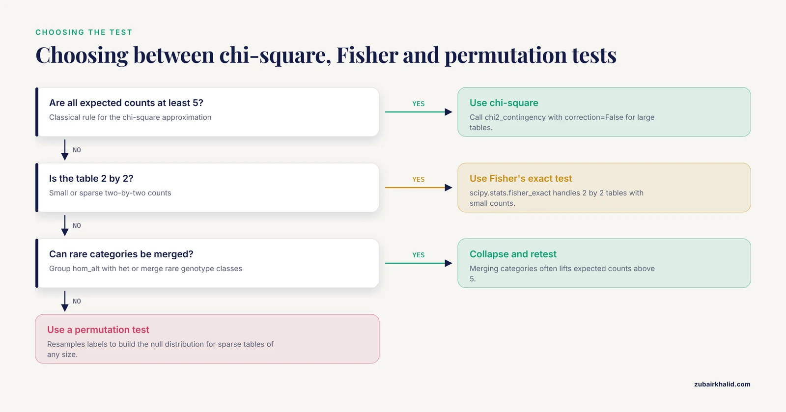
The chi-square distribution is an approximation, and the approximation is only trustworthy when expected counts are large enough. The standard rule, from classical statistics texts, is that all expected counts should be at least 5, and some sources relax this to no more than 20% of cells below 5 with no cell below 1. Check directly:
print(expected.min())          # smallest expected count
print((expected < 5).mean())   # fraction of cells below 5
For the worked table, the minimum expected count is 21, comfortably above the threshold, so the approximation is safe. When expected counts are too small, the standard fixes are:
- Collapse rare categories (for example, group hom_alt with het, or merge rare genotype classes).
- Use Fisher's exact test, available in SciPy for 2×2 tables as
scipy.stats.fisher_exact. - Use a permutation test, which resamples labels and builds the null distribution empirically. This is the go-to option for sparse genomic tables of any size.
Step 4: Hardy-Weinberg Goodness-of-Fit in Python
Hardy-Weinberg equilibrium (HWE) predicts genotype frequencies from allele frequencies when a population mates randomly and evolutionary forces are absent. Deviations can flag genotyping error, population structure, or selection, and HWE filtering is a standard QC step in genome-wide association pipelines.
Suppose you observed 40 AA, 45 Aa, and 15 aa among 100 individuals. Compute allele frequencies, derive expected counts, and run scipy.stats.chisquare:
from scipy.stats import chisquare

observed = np.array([40, 45, 15])          # AA, Aa, aa
n = observed.sum()                          # 100 individuals
p_A = (2 * observed + observed[1]) / (2 * n)   # 0.625
p_a = 1 - p_A                                     # 0.375

expected = np.array([
    p_A**2 * n,        # 39.0625
    2 * p_A * p_a * n, # 46.875
    p_a**2 * n,        # 14.0625
])

stat, pval = chisquare(f_obs=observed, f_exp=expected)
print(f"p_A = {p_A:.3f}, expected = {expected}")
print(f"chi2 = {stat:.4f}, p = {pval:.4f}")
Expected output:
p_A = 0.625, expected = [39.0625 46.875  14.0625]
chi2 = 0.1600, p = 0.6892
With p = 0.69, these counts are entirely consistent with Hardy-Weinberg proportions. Notice the degrees of freedom here: three genotype classes with the allele frequency p estimated from the data costs one df, so df = 3 - 1 - 1 = 1. chisquare assumes df = k - 1 by default, so for HWE you are responsible for remembering the extra df spent on estimation. With df = 1 and a single degree-of-freedom test, some analysts also apply a continuity correction, though for HWE filtering most pipelines report the uncorrected statistic.
Step 5: Quantify Effect Size and Inspect Residuals
A p-value tells you whether an association exists, not how strong it is. With large cohorts, trivially small genotype differences produce tiny p-values. Two quantities fix this.
Cramér's V measures association strength for tables of any size, on a 0 to 1 scale:
n = table.sum()
r, c = table.shape
cramers_v = np.sqrt(chi2 / (n * (min(r - 1, c - 1))))
print(f"Cramer's V = {cramers_v:.3f}")
For the worked example: V = √(21.591 / (200 × 1)) = 0.329. That is a moderate association, strong by genomewide SNP standards where most variants show V near 0.
Standardized (Pearson) residuals show which cells drive the deviation:
residuals = (table - expected) / np.sqrt(expected)
print(np.round(residuals, 2))
Output:
[[-1.96 -0.93  2.47]
 [ 1.96  0.93 -2.47]]
Cases carry fewer AA and more aa genotypes than expected (residuals beyond roughly ±2 are notable). This is the interpretive payoff of the test, and it takes one line.
Step 6: Scale the Workflow Across Many Variants
Genomewide scans repeat the test once per variant. The structure is a loop with a results list:
import numpy as np
from scipy.stats import chi2_contingency

def snp_chi2(counts, correction=False):
    """counts: array of shape (2, 3), rows case/control, cols AA/Aa/aa."""
    if counts.min(axis=1).sum() == 0:
        return np.nan, np.nan, np.nan   # skip monomorphic or empty rows
    chi2, p, dof, expected = chi2_contingency(counts, correction=correction)
    if expected.min() < 5:
        return chi2, p, np.nan          # flag low-expected-count variants
    n = counts.sum()
    v = np.sqrt(chi2 / (n * (min(counts.shape) - 1)))
    return chi2, p, v

results = []
for variant_counts in all_variant_tables:      # your iterable of (2,3) arrays
    results.append(snp_chi2(variant_counts))

results = pd.DataFrame(results, columns=["chi2", "p", "cramers_v"])
results["p_bonferroni"] = np.minimum(results["p"] * len(results), 1.0)
The Bonferroni adjustment multiplies each p-value by the number of tests (or equivalently compares against α/m, so with 500,000 SNPs the threshold is 1 × 10⁻⁷). For a less conservative alternative, the Benjamini-Hochberg false discovery rate procedure is available through statsmodels.stats.multitest.multipletests with method='fdr_bh'. For the smallest p-value out of a million tests to survive Bonferroni correction at α = 0.05, the raw p must be below 5 × 10⁻⁸, which is exactly the conventional genomewide significance threshold.
Key Parameters and Formulas at a Glance
| Item | Value or formula | When it matters | ||
|---|---|---|---|---|
| χ² statistic | Σ (O - E)² / E | Both independence and goodness-of-fit tests | ||
| Expected count (independence) | (row total × column total) / grand total | Computed automatically by chi2_contingency | ||
| Expected count (HWE) | p²·N, 2pq·N, q²·N | HWE filtering of variants | ||
| df (independence) | (rows - 1) × (cols - 1) | Set automatically by SciPy | ||
| df (goodness of fit) | k - 1 - (estimated parameters) | HWE spends 1 df on allele frequency p | ||
| Yates correction | subtract 0.5 from each \ | O - E\ | 2×2 tables only, correction=True default in SciPy | |
| Minimum expected count | all cells ≥ 5 (classical rule) | Decide between χ² and exact or permutation tests | ||
| Cramér's V | √(χ² / (N × min(r-1, c-1))) | Effect size, 0 to 1 scale | ||
| Pearson residual | (O - E) / √E | Locating which cells drive the association | ||
| Bonferroni threshold | α / number of tests | Genomewide scans, typically 5 × 10⁻⁸ |
Checking That Your Result Is Correct
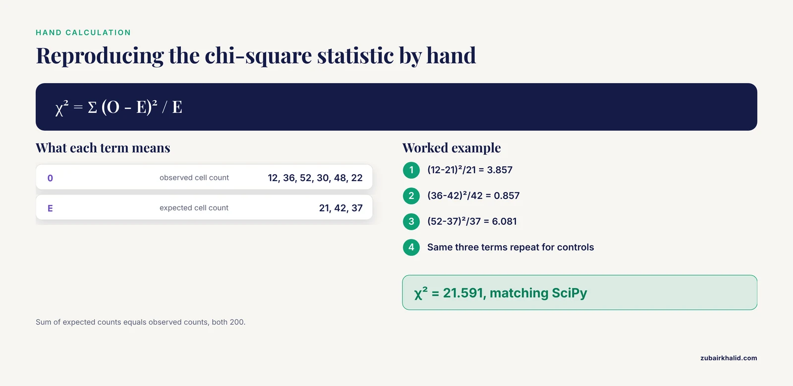
Verify the machinery once with a hand calculation before you trust it across a pipeline. For the worked 2×3 table, every expected count is a clean integer (21, 42, 37), so the statistic is easy to reproduce with a calculator:
χ² = (12-21)²/21 + (36-42)²/42 + (52-37)²/37
   + (30-21)²/21 + (48-42)²/42 + (22-37)²/37
   = 3.857 + 0.857 + 6.081 + 3.857 + 0.857 + 6.081
   = 21.591
That matches the SciPy output exactly. Three further checks are worth building into any pipeline.
First, cross-check small or borderline tables with Fisher's exact test. If chi-square and exact test disagree on significance, trust the exact test for small counts. Second, confirm that the sum of expected counts equals the sum of observed counts (both equal the grand total, 200 here), which catches transcription errors in the input table. Third, when you embed chi-square logic inside an automated QC or filtering step, require that the decision rule be explicit and fixed in advance. The SEAOP toolbox illustrates the pattern: candidate results are aggregated by a chi-square test held at a 95% confidence level, so the acceptance criterion is stated, reproducible, and not adjusted after seeing the data [1]. A fixed confidence level written into the pipeline beats an ad hoc threshold chosen while looking at the results.
A note on what "correct" means: the test tells you whether counts deviate from a null expectation. It does not by itself establish causation, direction, or mechanism. Those come from study design, replication, and downstream biological validation.
Working with Biopython and Standard Formats
A biopython tutorial on this topic usually starts one step upstream of the statistics, with getting counts out of standard file formats. Biopython handles the formats, SciPy handles the test, and the two connect through plain count arrays.
For codon usage studies, parse coding sequences with Bio.SeqIO, count codons, and compare the observed distribution against an expected distribution with scipy.stats.chisquare. A compact sketch:
from Bio import SeqIO
from collections import Counter

codons = Counter()
for record in SeqIO.parse("cds.fasta", "fasta"):
    seq = str(record.seq).upper()
    for i in range(0, len(seq) - 2, 3):
        codon = seq[i:i+3]
        if set(codon) <= set("ACGT") and codon not in ("TGA", "TAA", "TAG"):
            codons[codon] += 1

print(codons.most_common(5))
You can then collapse the 61 sense codons into biologically meaningful categories (GC-ending versus AT-ending, or by amino acid) and test the resulting table against an expected distribution. Collapsing matters here for the same reason it matters in Step 3: 61 codon categories with sparse counts would violate the expected-count rule badly.
Biopython also reads population-genetic formats such as GenePop through its Bio.PopGen modules, which is convenient when exchanging data with population genetics software. For VCF files at scale, dedicated parsers such as pysam or cyvcf2 are faster than line-by-line parsing, but the aggregation step, pd.crosstab on genotype and status, stays the same.
Common Mistakes and Limitations
Applying the chi-square test to continuous data. The test needs counts in categories. If your "genomic" data are expression levels, methylation beta values, or read depths, chi-square is the wrong tool. Continuous measurements call for t-tests, Wilcoxon tests, or regression. Bin a continuous variable only with a stated, pre-planned rationale.
Ignoring the expected-count rule. Rare variant analyses routinely produce tables where one genotype class has fewer than 5 expected observations. The p-value from a chi-square test in that regime is unreliable. Collapsing categories, switching to Fisher's exact test for 2×2 tables, or using a permutation test are the standard remedies.
Leaving the Yates correction on for large 2×2 tables. SciPy's default is correction=True for 2×2 input. On a table with thousands of samples, the correction biases the test toward non-significance. Genomic association testing conventionally uses correction=False, reserving the correction for small-sample situations.
Forgetting multiple testing. A single chi-square test at α = 0.05 has a 5% false positive rate. Run it across 500,000 variants and you expect roughly 25,000 false positives at that threshold. Bonferroni or FDR correction is not optional in genomewide scans. This is also why embedded statistical gates in pipelines use explicitly fixed confidence levels, as SEAOP does with its 95% confidence aggregation step [1].
Treating related individuals as independent. The chi-square test assumes independent observations. Family-based cohort data violate this, inflating the statistic and producing spurious significance. Use family-based tests or mixed models for related samples instead, and reserve plain chi-square for unrelated individuals.
Confusing the two degrees-of-freedom conventions. A HWE goodness-of-fit test with three genotype classes has df = 1, not 2, because one df is spent estimating the allele frequency from the same data. scipy.stats.chisquare defaults to df = k - 1 and will not make this adjustment for you. Passing ddof=1 to chisquare subtracts the additional df.
Running chi-square on allele frequencies instead of counts. Pooling samples and testing the frequency 0.37 against 0.41 discards the sample size information that the test depends on. Always test counts.
Zero rows or columns crash the function. If a genotype class is absent in both cases and controls, SciPy raises:
ValueError: The internally computed table of expected frequencies has a zero element at index (x, y).The fix is to drop the empty column before testing, with table[:, table.sum(axis=0) > 0] for NumPy arrays.
Overinterpreting significance. A significant χ² on 100,000 samples can correspond to a Cramér's V of 0.01, an association so weak it has no practical meaning. Report effect size alongside every p-value.
The chi-square test assumes unstructured sampling. Population stratification, batch effects, and batch-correlated ascertainment can all create count differences that have nothing to do with the biological question. Within-stratum analyses or structured methods are the appropriate response when stratification is suspected.
Finally, an individual analysis rarely settles a biological question on its own. Chi-square results belong inside a workflow that includes replication, effect-size estimation, and domain expertise, and specific research questions deserve input from a collaborator with the relevant statistical and biological background.
Frequently Asked Questions
When should I use a chi-square test instead of Fisher's exact test in genomics?
Use chi-square when expected counts in every cell are at least 5 and your tables are large, which is typical for cohort-scale genotype counts. Use Fisher's exact test for 2×2 tables with small or sparse counts, and permutation tests for sparse tables of any size.
How do I run a chi-square test on SNP genotype counts in Python?
Arrange the counts as a NumPy array with cases and controls as rows and genotypes as columns, then call scipy.stats.chi2_contingency(table, correction=False). The call returns the χ² statistic, p-value, degrees of freedom, and expected counts in one step.
What is the minimum expected count rule for a chi-square test?
The classical rule requires every expected cell count to be at least 5. A common relaxation allows up to 20% of cells below 5 provided none falls below 1. If your table fails, collapse categories or switch to an exact or permutation test.
Should I use the Yates correction for genomic 2×2 tables?
Usually no. The Yates correction is appropriate for small samples with unbalanced margins, but large genomic tables should be tested with correction=False to avoid unnecessary conservatism. SciPy applies the correction by default for 2×2 input, so you must disable it explicitly.
How do I handle millions of SNPs in one chi-square scan?
Run the test in a loop or vectorized batch, then correct for multiple testing. Bonferroni at α divided by the number of tests gives the standard 5 × 10⁻⁸ threshold for roughly one million variants, and Benjamini-Hochberg FDR control offers a less conservative alternative.
Can I test Hardy-Weinberg equilibrium with scipy.stats?
Yes. Compute allele frequencies from genotype counts, build expected counts as p²·N, 2pq·N, and q²·N, and pass observed and expected counts to scipy.stats.chisquare. Remember the degrees of freedom are 1 for a diallelic marker because one df is spent estimating the allele frequency.
What Python libraries do I need for chi-square tests in bioinformatics?
NumPy, SciPy, and pandas cover the core workflow, since scipy.stats.chi2_contingency and scipy.stats.chisquare perform the tests and pandas aggregates raw calls into count tables. Biopython helps when your data start in formats such as FASTA or GenePop.
How do I interpret the chi-square statistic versus the p-value?
The statistic measures how far observed counts sit from expected counts in standardized units, and the p-value converts it into the probability of seeing a deviation that large under the null hypothesis. A large statistic with a small p-value means real deviation, while the effect size (Cramér's V) tells you how much the variables actually associate.