How to Speed Up Genomic Data Analysis in R with Parallel Computing
By Dr. Zubair Khalid, DVM, MS, PhD ·

By the end of this article you will be able to take a slow loop in an R genomics script, measure how long it actually takes, parallelize it correctly with parallel, foreach, or BiocParallel, verify that the parallel result matches the serial result, and diagnose the failures that most commonly stop people, including worker crashes, memory exhaustion, and seeds that silently change your p-values. You will also know when parallel computing is the wrong tool and when out-of-memory Bioconductor containers or a separate compiled program will get you further.
Before you start, have the following on hand:
- R 4.2 or newer. Check with
R.version.string. - The
parallelpackage, which ships with base R, andforeachplusdoParallelfrom CRAN. - Bioconductor and
BiocParallelif you work with Bioconductor objects such asGRanges,SummarizedExperiment, orDelayedArray. - A machine with at least 2 physical cores, ideally 8 or more, and enough free RAM that you can hold your largest intermediate object at least once per worker.
- A realistic task to practice on, such as permutation testing, per-chromosome summaries, or marker-by-marker regressions.
R is one of the standard environments for r for bioinformatics work, and the Bioconductor project provides the dominant package ecosystem for sequencing and genomics analysis. The scalability problem is well documented. A review of scalable genomics with R and Bioconductor identifies four general strategies for large genomic data, namely restrictive queries, compression, iteration, and parallel computing [1]. This article focuses on the fourth strategy and shows how to combine it with the other three, because parallelizing a naive script that loads everything into memory usually just runs out of RAM faster.
Why Genomic Workflows in R Get Slow
Three properties of typical genomic data cause most of the pain:
- Many independent units. A GWAS summary file has one row per marker. A single-cell matrix has thousands of genes or cells. Analyses that treat each row, gene, chromosome, or permutation separately are naturally parallelizable, and this is where you get the biggest wins.
- Data larger than memory. A plink binary genotype file with 500,000 individuals and 1 million markers is on the order of hundreds of gigabytes. R's default data frames cannot hold that. The BGData suite was built precisely for this situation, providing a matrix-like interface for plink
.bedfiles, linked arrays that span multiple files, and parallel computing methods that work on very large datasets without loading everything into memory [2]. - Interpreted loops. R interprets each iteration of a
forloop. Vectorized operations and compiled extensions are faster, but many genomic algorithms are inherently iterative, such as Markov chain Monte Carlo samplers for Bayesian marker-effect models [3].
There is also an honest alternative worth stating up front. BESSiE, a program for linear model BLUP and Bayesian MCMC analysis of large-scale genomic data, exists partly because script-based environments like R may struggle with very large marker matrices or cannot exploit model structure that saves computing time [3]. If your analysis is a standard Bayesian genomic prediction model, a purpose-built command-line tool may beat anything you write in R. Use parallel R where it fits, and use specialized compiled tools where they fit better. PRSice-2, for example, was written specifically because biobank-scale polygenic risk score analyses required more efficient and scalable software than earlier options, and it was benchmarked as faster and more memory-efficient than PRSice-1, LDpred, and lassosum [4].
The rest of this article is a practical guide to getting the most out of R itself.
A Step-by-Step Parallel Computing Workflow in R for Genomics
This section is the core walkthrough. It doubles as a short Bioconductor tutorial for BiocParallel, since that package is the standard way Bioconductor packages accept parallel backends.
Step 1: Check Your Environment and Core Count
Run this first so you know what hardware you are actually working with.
R.version.string
parallel::detectCores()
parallel::detectCores(logical = TRUE)
system("free -h 2>/dev/null || vm_stat 2>/dev/null || echo 'check RAM manually'")
Expected output looks like this on an 8-core laptop with hyperthreading:
[3] "R version 4.3.2 (2023-10-31)"
[3] 8
[3] 16
detectCores() without arguments returns physical cores. logical = TRUE returns hardware threads. Plan your worker count from physical cores, not logical threads, for compute-bound work. Record these numbers, because every later decision depends on them.
Step 2: Benchmark the Serial Version Before Parallelizing Anything
Never parallelize blind. Measure the serial runtime first, because it becomes your baseline for deciding whether the parallel version is actually helping.
Create a realistic toy task that mirrors genomics work, an empirical permutation test for a SNP-phenotype association:
set.seed(42)
n <- 5000
x <- rbinom(n, 2, 0.3)          # SNP genotypes 0, 1, 2
y <- 0.05 * x + rnorm(n)        # quantitative phenotype

one_perm <- function(i) {
  abs(cor(x, sample(y)))
}

system.time(perm_serial <- vapply(1:10000, one_perm, numeric(1)))
Expected output on a mid-range laptop:
   user  system elapsed
  6.411   0.208   6.631
Six seconds for one marker. A chromosome with 80,000 markers at this rate would take roughly six days serial. That gap is exactly why parallel computing in R genomics pipelines matters, and also why the fastest real-world pipelines offload whole stages to compiled tools rather than looping in R at all.
Step 3: Use parallel::mclapply for Embarrassingly Parallel Work on Unix and macOS
Tasks where each element is independent of the others are called embarrassingly parallel. Permutations, per-chromosome summaries, and per-gene tests all qualify. On Linux and macOS, mclapply forks the current R session, which is cheap because workers share memory copy-on-write.
library(parallel)
n_cores <- detectCores() - 1

system.time(perm_par <- mclapply(1:10000, one_perm, mc.cores = n_cores))
perm_par <- unlist(perm_par)
Expected output:
   user  system elapsed
 42.971   1.522   1.487
Two things to notice. First, user time exceeds elapsed time because multiple cores are working at once. Second, this is not a perfect 8-fold speedup from the 6.6-second baseline. Each worker pays overhead for forking and collecting results, and sample() is fast enough that per-call overhead is a real fraction of total work. This pattern, where observed speedup is less than the number of cores, is normal. The parallel biocomputing literature reports near-linear speedup for computationally intensive tasks such as eQTL scans on a MOSIX cluster, while noting that the level of improvement always depends on the nature of the algorithm [5]. A review of the SPRINT parallel R package on Amazon EC2 reached the same conclusion, finding good scalable performance whose level depended on the algorithm, and even found that deliberately underutilizing resources could improve time to result [6].
Two mclapply parameters matter most:
mc.cores: the number of worker processes. Set it to physical cores minus 1 so your machine stays responsive.mc.preschedule: defaults toTRUE, which pre-splits the range of jobs into roughlymc.coreschunks. Set it toFALSEwhen individual jobs have wildly variable runtimes, for example when some genes have far more transcripts to process than others.
Step 4: Use parLapply and foreach on Windows or for Cluster-Style Control
Forking does not exist on Windows, and on any platform you may want explicit control over worker setup. makePSOCKcluster starts worker R sessions over socket connections and works everywhere.
library(parallel)
cl <- makeCluster(7)              # 7 workers on an 8-core machine
clusterExport(cl, varlist = c("x", "y", "one_perm"))

system.time(perm_snow <- parLapply(cl, 1:10000, one_perm))
perm_snow <- unlist(perm_snow)

stopCluster(cl)                   # always do this, or workers linger
Expected output:
   user  system elapsed
  0.013   0.004   1.892
Elapsed time is what counts here. User time stays near zero because the main process is idle while workers compute.
The foreach package gives you the same mechanics with loop syntax that many find easier to read, and it is the standard entry point for reproducible parallel scripts:
library(foreach)
library(doParallel)

registerDoParallel(cores = 7)

system.time(
  perm_foreach <- foreach(i = 1:10000, .combine = "c") %dopar% {
    one_perm(i)
  }
)
Expected output:
   user  system elapsed
  0.897   0.663   1.761
Key parameters:
.combine = "c"concatenates each worker's returns into one numeric vector. Use"rbind"for data frames,"+"for sums, and"list"when you need order-preserving lists.registerDoParallel(cores = n)sets the backend. Calling it once at the top of a script keeps the rest of the code backend-agnostic.foreach(..., .packages = c("dplyr", "limma"))loads packages inside each worker. This is the single most forgotten parameter in foreach code.
Step 5: Use BiocParallel Inside Bioconductor Workflows
Bioconductor packages accept a BPPARAM argument, and BiocParallel routes it to the right backend for your platform. This is the level of abstraction you want for long-lived genomics code, because the same script then runs serially on a laptop and in parallel on an HPC node with no edits.
library(BiocParallel)

# Multicore for Unix/macOS, Snow for Windows, Serial for debugging
param_unix  <- MulticoreParam(workers = 7, RNGseed = 42)
param_win   <- SnowParam(workers = 7, RNGseed = 42)
param_debug <- SerialParam()

system.time(
  perm_bioc <- bplapply(1:10000, one_perm, BPPARAM = param_unix)
)
Expected output:
   user  system elapsed
 44.103   1.871   1.596
Choose backends with this logic:
MulticoreParamforks, so it is fastest on Unix and macOS but fails on Windows.SnowParamspawns socket workers, works everywhere, and is the portable choice for scripts shared across platforms.SerialParamruns everything in one process. Keep it available as a debugging switch.DoparParammakesBiocParallelrespect whatever backend you registered withforeach.
RNGseed deserves its own emphasis. Permutation tests are random-number hungry, and reproducibility requires that workers draw from controlled streams. We return to this in the verification section.
Step 6: Chunk Your Jobs Instead of Dispatching One Task per Element
Dispatching 10,000 separate one-permutation jobs creates per-task communication overhead. Split the work into chunks roughly equal to or somewhat larger than the number of workers:
n_perms <- 10000
chunked <- split(1:n_perms, cut(1:n_perms, n_cores, labels = FALSE))

chunk_fun <- function(idx) {
  vapply(idx, one_perm, numeric(1))
}

system.time(perm_chunked <- unlist(mclapply(chunked, chunk_fun, mc.cores = n_cores)))
Expected output:
   user  system elapsed
 43.220   0.914   1.404
On this small example chunking saves about 10 percent. On jobs with heavier per-task setup, such as reading a file or fitting a mixed model, chunking routinely saves far more. The general principle, iterate over data in controlled blocks rather than materializing everything at once, is one of the four scalability strategies identified in the R and Bioconductor scalability review [1].
Step 7: Handle Data That Does Not Fit in Memory
When the genotype matrix itself is the bottleneck, parallelizing the loop is not enough because you cannot even load the data. Two approaches work.
The first is file-backed arrays in Bioconductor. DelayedArray and related classes keep data on disk and realize only the slices a computation touches, which pairs naturally with chunked parallel iteration [1].
The second is the BGData suite, which provides a matrix-like interface to plink .bed files and linked arrays spanning multiple files, with built-in parallel methods designed to carry out computations on very large datasets without loading the entire data into memory [2]. A typical pattern:
# install.packages("BGData")
library(BGData)

# genotypes stay on disk, only chunks are pulled into RAM
bg <- BGData("my_cohort.bed")

chunked_summary <- chunkedApply(bg, margin = 2, chunk.size = 10000,
                                FUN = colMeans, n.cores = 7)
The exact function names and arguments vary by BGData version, so run ?BGData and read the vignette for your installed release before writing production code. The structural idea, apply a function over chunks of an on-disk matrix with several cores, is what matters and transfers directly to UK Biobank-scale data [2].
Step 8: Scale Out When a Single Machine Is Not Enough
When one node cannot hold the data or finish in reasonable time, you move from one machine with many cores to many machines. Two well-documented paths exist.
On a traditional cluster or a low-cost commodity cluster, the workflow manager matters as much as the parallel backend. DolphinNext is a distributed processing platform for high-throughput genomics built to provide the combination of parallelism, portability, flexibility, and reproducibility that research pipelines require, with a graphical interface for building complex pipelines [7]. Treat pipeline-level parallelism, running independent samples or chromosomes as separate jobs on a scheduler, as a complement to in-session parallelism, not a replacement.
In the cloud, the SPRINT experience on Amazon EC2 is instructive. SPRINT is an R package giving genomics researchers straightforward access to parallel implementations of correlation, permutation testing, partitioning around medoids, and a multi-purpose papply, and the authors benchmarked these on Amazon EC2 from multiple regions, finding that end-user location mattered for cost and that underutilized resources could improve time to result [6]. The practical lesson is that cloud billing makes worker efficiency directly measurable in dollars, so chunking and avoiding oversubscription pay for themselves.
A third path is to push the heaviest computation into purpose-built compiled tools and keep R for orchestration. Parallel-META 3, a metagenomic comparison toolkit implemented in C and C++ with R integration, processed 5,337 samples totaling over 1.1 billion sequences with lower memory usage and much faster speed than QIIME and PICRUSt while producing similar results [8]. RGMQL takes a related approach for genomic region data, letting R/Bioconductor code delegate scalable processing to the GMQL engine, including remote cloud services [9].
Choosing a Parallel Backend in R
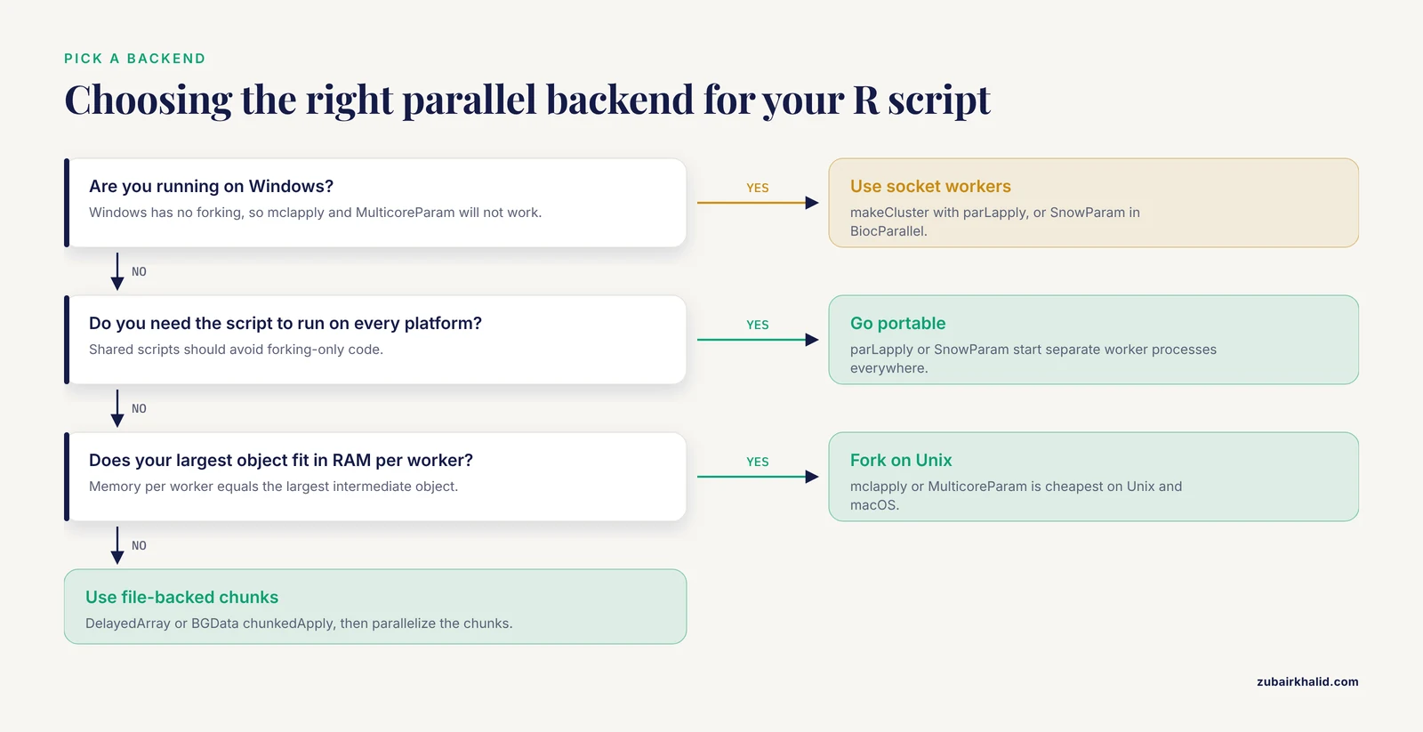
The table below summarizes the main options and when each is the right choice.
| Backend | Function | Platforms | Best for | Overhead |
|---|---|---|---|---|
| Forking | mclapply, MulticoreParam | Unix, macOS | Many short independent tasks on one machine | Very low |
| Socket cluster | makeCluster, parLapply, SnowParam | All, including Windows | Portable scripts, explicit worker control | Moderate |
| foreach | foreach with %dopar% | Depends on registered backend | Readable loops, reproducible scripts | Moderate |
| Chunked apply | chunkedApply in BGData, custom splits | All | Data larger than RAM, plink .bed files | Low per chunk |
| External tools | BESSiE, PRSice-2, Parallel-META 3 | Linux primarily | Whole pipeline stages at biobank scale | One-time setup |
The pattern across published benchmarks is consistent. Purpose-built parallel implementations of specific algorithms, such as parmigene for mutual information network inference, deliver large gains because they parallelize the algorithm itself rather than a generic loop. parmigene uses a k-nearest-neighbor mutual information estimator and a parallel computing paradigm to reconstruct large gene regulatory networks at strikingly lower computational cost than earlier software [10]. Similarly, the cross-trait penalized regression method CTPR introduced a novel parallel computing algorithm specifically to make multi-trait polygenic prediction feasible on biobank-scale GWAS data, applying it to roughly 1 million SNPs from 456,837 UK Biobank participants [11]. When a parallel implementation of your exact algorithm exists, use it before writing your own.
Common Errors and Their Exact Fixes
"could not find function" inside workers
Error in one_perm(idx) : could not find function "sample"Workers start as fresh R sessions or forks of your session at export time. Fix by exporting everything they need:
clusterExport(cl, varlist = c("x", "y", "one_perm"))
clusterEvalQ(cl, library(matrixStats))   # packages too
With foreach, use .export and .packages arguments instead. With mclapply, forking usually inherits your workspace, which is why errors of this type tend to appear only after you switch backends.
mclapply returns NULL values
Warning message:
In mclapply(...) : all scheduled cores encountered errors in user code
mclapply fails silently by default, returning NULL for failed elements. Check attr(result, "failed") to see which jobs failed, then re-run a single job serially to surface the real error message. On macOS, RStudio and forked processes conflict, so if workers die immediately, run the script with Rscript in a terminal or switch to SnowParam.
"cannot allocate vector of size"
Error: cannot allocate vector of size 12.0 GbYou multiplied memory by your worker count. With 7 workers each holding a 2 Gb intermediate, you need roughly 14 Gb free, not 2. Fixes in order of preference, reduce chunk size, reduce worker count, switch to a file-backed container such as those in BGData that compute on chunks without loading the full data [2], or subset with restrictive queries so only needed rows and columns are ever materialized [1].
Results differ between serial and parallel runs
If permutation results change when you switch to parallel code, the random number streams changed. Fix with proper parallel RNG:
cl <- makeCluster(7)
clusterSetRNGStream(cl, iseed = 42)      # independent streams per worker
or with RNGseed = 42 in MulticoreParam and SnowParam. Note that the parallel result with a proper RNG is not identical to the serial result with set.seed, because the draws differ. It is statistically equivalent and reproducible, which is what you actually need.
Errors 1 through 7 of 8 reported by BiocParallel
Error: BiocParallel errors
  7 remote errors, element index: 2, 3, 4, 5, 6, 7, 8
BiocParallel collects worker errors and reports their indices. Re-run the failing index with SerialParam() to get the full traceback. A single failing element, for example a gene with all-zero counts, will otherwise kill an entire batch repeatedly.
Performance gets worse with more cores
This is almost always oversubscription. Linear algebra libraries like OpenBLAS or MKL already use multiple threads, so 7 workers each spawning multithreaded BLAS calls means dozens of threads fighting over 8 cores. Cap BLAS threads before registering workers:
library(RhpcBLASctl)
blas_set_num_threads(1)
Then each worker does its own linear algebra single-threaded and the outer parallelism is clean.
How to Verify Your Parallel Results Are Correct
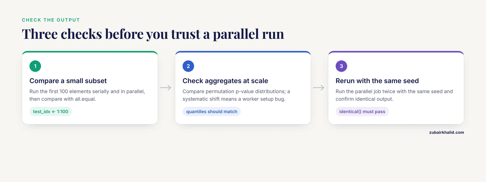
Parallelization should change runtime, never results. Verify with three checks on every new pipeline:
- Subset equivalence. Run the first 100 elements serially and in parallel, then compare:
test_idx <- 1:100
stopifnot(
  isTRUE(all.equal(
    vapply(test_idx, one_perm, numeric(1)),
    unlist(mclapply(test_idx, one_perm, mc.cores = 4))
  ))
)- Aggregate checks at full scale. For permutation p-values, compare distributions. Serial and parallel versions with valid independent RNG streams should give nearly identical quantiles, and any systematic shift means a bug in your worker setup.
- Seed reproducibility. Run the parallel job twice with the same seed and confirm
identical()output. If it fails, you are consuming RNG non-deterministically across workers.
This step matters more in genomics than in most R work because downstream conclusions often rest on which markers cross a significance threshold. The GWAtoolbox package was built around exactly this quality-control mindset for GWAS meta-analysis, checking data formatting, result quality, and cross-study consistency, and its workflow can QC any number of files in a matter of minutes [12]. Build the equivalent habit into your own parallel code before trusting its output.
Common Mistakes and Limitations
- Parallelizing before profiling. If 95 percent of runtime is one file read or one
merge(), parallelizing the loop around it changes nothing. Profile withprofvis()orsystem.timearound each stage first. - Ignoring memory as the real constraint. Worker counts are chosen by RAM as often as by cores. Memory per worker equals the largest intermediate object your function creates, and exceeding it crashes workers with unhelpful errors. BGData was created specifically because even parallel R code fails when the data cannot be loaded at all [2].
- Overwriting
mc.coreswith logical thread counts. Sixteen hyperthreads are not sixteen fast cores. Compute-bound genomic tasks usually peak at physical core count. - Forking in interactive IDE sessions on macOS.
mclapplyfrom within some GUI environments hangs or crashes. The standard practice is to run production parallel scripts withRscriptand reserve interactive testing for small batches withSerialParam. - Assuming all algorithms parallelize. MCMC chains are sequential within a chain. The standard speedup is running independent chains in parallel, not splitting one chain. BESSiE handles the marker-effect MCMC algorithms themselves in compiled code rather than trying to parallelize the chain internally [3].
- Losing reproducibility through unseeded parallel RNG. Permutation-based genomics is especially vulnerable. Use
clusterSetRNGStreamorRNGseedevery time. - Parallelizing I/O. Seven workers reading the same large file can be slower than one worker reading it once and distributing the result. Read once, then fork.
- Expecting linear speedup forever. Speedup depends on the fraction of work that is truly parallel and on communication overhead. Benchmarks of parallel R in genomics consistently show algorithm-dependent scaling [6] [5].
A final limitation applies to the analysis itself. Parallel computing accelerates computation, it does not validate model assumptions, correct batch effects, or substitute for domain judgment about a specific dataset, and individual research questions need that judgment applied case by case.
Tips That Compound Over a Project
- Standardize on
BPPARAMarguments in your own functions. Accepting aBPPARAM = SerialParam()default makes every function you write debuggable serially and scalable in parallel with one argument. - Log worker failures with indices. When a remote worker fails at element 4,312, you need to know what made element 4,312 special. Wrap worker functions in
tryCatchand return the error message alongside the index. - Match the parallel unit to the science. Per-chromosome and per-gene chunks make results interpretable and let you resume partial failures. Arbitrary index chunks do neither.
- Combine parallelism with iteration and restrictive queries. The Bioconductor scalability strategies, restrictive queries, compression, iteration, and parallel computing, work best together. Query only the genomic ranges you need, iterate in chunks, and parallelize the chunks [1].
- Reinvest saved time in QC. Faster pipelines tempt people to skip validation. GWAtoolbox-style automated QC exists so that speed and rigor can coexist, checking format, quality, and consistency across studies in minutes [12].
Where to Go Next
Once the in-session parallelism here is working, three directions extend your reach. First, move pipeline-level orchestration to a workflow system so independent samples run as scheduler jobs, following the parallelism, portability, and reproducibility principles articulated for platforms like DolphinNext [7]. Second, adopt Bioconductor's out-of-memory containers for data that grows past RAM, the approach demonstrated at UK Biobank scale with BGData [2]. Third, identify whether a dedicated parallel tool already exists for your bottleneck, whether that is mutual information networks [10], polygenic risk scores [4], metagenomic comparison [8], or genomic region queries delegated to a remote engine [9]. Writing less R and orchestrating more compiled parallel code is usually the single biggest win available.
The methods in this article are the mainstream toolkit of modern r for bioinformatics practice. Master them on a small permutation test before you point them at a biobank, and benchmark every change, because the honest measure of parallel work is elapsed time and correct results, nothing else.
Frequently Asked Questions
How many cores should I use for parallel R genomics work?
Use physical cores minus one for interactive machines, all physical cores on a dedicated compute node, and cap BLAS threads at one per worker to avoid oversubscription. The optimal count is always empirical, so benchmark at 2, 4, and your maximum and keep the fastest setting.
Does parallelizing my analysis change my p-values or results?
It should not, as long as you use proper parallel random number streams with clusterSetRNGStream or RNGseed. The numbers may differ from a serial run because the random draws differ, but the statistical distribution and conclusions are equivalent, and reruns with the same seed are reproducible.
Should I use mclapply or parLapply?
Use mclapply on Unix and macOS because forking is nearly free, and use parLapply on Windows or when you need explicit control over the worker environment. mclapply fails silently on worker errors, so check for NULL elements, while parLapply propagates errors to the main session.
Does parallel R work the same way on Windows?
No, because Windows has no forking. Use makeCluster with parLapply, or SnowParam with BiocParallel, both of which start separate worker processes over socket connections. Code that works this way is portable to every platform, which makes it the safer default for shared scripts.
What if my genomic data does not fit in RAM at all?
Use file-backed containers instead of loading everything. Bioconductor's DelayedArray classes realize only requested slices, and the BGData suite provides a matrix-like interface to plink .bed files with parallel methods that compute on very large datasets in chunks [2]. Parallelize the chunk iteration, not the data loading.
Is BiocParallel required for Bioconductor packages?
It is not required for all packages, but it is the standard mechanism they use to accept parallel backends, so learning it pays off across the ecosystem. Many Bioconductor functions accept a BPPARAM argument, and passing SerialParam() gives you a reliable serial debugging mode for the same code.
How do I speed up code that is not embarrassingly parallel?
Start by checking whether an existing parallel implementation of the algorithm exists, since dedicated tools such as parmigene for gene network inference or CTPR for multi-trait prediction were built for exactly this problem [10] [11]. If none exists, look for parallelism at a higher level, such as independent chains, cross-validation folds, or samples, and consider moving the bottleneck to compiled code.
Should I move my R genomics pipeline to the cloud?
Consider it when data volume or deadlines exceed your local hardware, since parallel R packages have been benchmarked successfully on Amazon EC2 with good scalable performance [6]. Factor in data transfer time and per-hour billing, which makes inefficient worker setups cost real money, and prefer purpose-built scalable services for whole pipeline stages when they exist [9].
Sources
- Scalable Genomics with R and Bioconductor.
- BGData - A Suite of R Packages for Genomic Analysis with Big Data.
- BESSiE: a software for linear model BLUP and Bayesian MCMC analysis of large-scale genomic data.
- PRSice-2: Polygenic Risk Score software for biobank-scale data.
- Parallel biocomputing.
- Exploiting parallel R in the cloud with SPRINT.
- DolphinNext: a distributed data processing platform for high throughput genomics.
- Parallel-META 3: Comprehensive taxonomical and functional analysis platform for efficient comparison of microbial communities.
- RGMQL: scalable and interoperable computing of heterogeneous omics big data and metadata in R/Bioconductor.
- parmigene--a parallel R package for mutual information estimation and gene network reconstruction.
- Efficient cross-trait penalized regression increases prediction accuracy in large cohorts using secondary phenotypes.
- GWAtoolbox: an R package for fast quality control and handling of genome-wide association studies meta-analysis data.