Outlier Samples Ruining Your PCA?

By Dr. Zubair Khalid, DVM, MS, PhD · 2026-11-11

By the end of this article you will be able to build a sample-level PCA from raw RNA-seq counts, quantify exactly which samples deviate using robust statistics instead of eyeballing, trace each outlier back to a concrete cause such as batch handling, low RNA quality, or a swapped library, and then make a defensible decision to remove, correct, or keep that sample. You will need R 4.3 or newer with the packages DESeq2, rrcov, ggplot2, and pheatmap, plus your raw count matrix and a sample sheet with real metadata. If you work upstream of the count matrix, keep FastQC and MultiQC reports on hand because per-sample sequencing metrics become part of the diagnosis.

PCA is usually the first plot reviewers and collaborators look at, and it is also the first plot a single bad library can ruin. The good news is that outlier detection in RNA-seq is a solved problem when you apply the right tools in the right order, and the workflow below follows the same logic published in the robust PCA literature for transcriptomic data [1].

Why One Bad Sample Can Distort the Whole PCA

Principal component analysis (PCA, a projection of high-dimensional data onto the directions of greatest variance) has no built-in resistance to extreme values. Each principal component is a weighted average of genes chosen to capture the largest possible variance. A sample whose expression profile is wildly off, whether from degradation, a batch reagent change, or a true biological extreme, inflates variance along its own direction. PC1 and PC2 then spend their budget describing that one sample instead of the biology you care about. The remaining samples collapse into a compressed blob, group structure shrinks, and every downstream plot built on those PCs inherits the distortion.

Two properties of RNA-seq make this worse than in most datasets. First, the data are extremely high-dimensional, often more than 20,000 genes, while a typical bulk experiment has fewer than a dozen samples per group. Second, extreme deviation of a sample from its treatment group can arise from technical variation during the multi-step library protocol or from genuine biological differences, and with few replicates these two causes are genuinely hard to separate [1]. This is why careful analysts do not treat PCA as a verdict. They treat it as a screening step that triggers quantitative follow-up.

There is also a statistical reason to prefer dedicated methods over squinting at a PCA plot. Classical PCA itself estimates the mean and covariance from all points, including the outliers, which pulls the fit toward the very samples you are trying to find. Robust statistics solve this by first fitting the majority of the data and then flagging points that deviate from that fit, an approach long used in chemometrics and engineering and now validated on RNA-seq data [1].

Before You Start

Install and load what you need in a fresh R session.

install.packages(c("BiocManager", "ggplot2", "pheatmap", "rrcov"))
BiocManager::install(c("DESeq2", "edgeR"))

library(DESeq2)
library(rrcov)
library(ggplot2)
library(pheatmap)

You should also have on hand:

A raw count matrix, genes in rows, samples in columns, integer counts from featureCounts, Salmon with tximport, or your quantifier of choice.
A sample sheet with sample IDs matching the count matrix column names, plus group labels, batch, library prep date, sequencing lane, extraction date, and RNA integrity values if measured.
Per-sample sequencing QC (mapping rate, duplicate rate, total reads) from your alignment or pseudoalignment step, since the upstream analysis pipeline you used defines what QC columns are available [2].

If any of that metadata is missing, request it before touching the plots. Outlier diagnosis without sample tracking information is guesswork.

Step-by-Step: Detecting an Outlier Sample in RNA-Seq PCA

This walkthrough assumes six samples, three control and three treated, stored as counts.csv (genes by rows, samples by columns) and coldata.csv (samples by rows). Adjust numbers as needed. Your output numbers will differ from the examples shown.

Step 1. Import the counts and confirm the sample sheet

cts <- read.csv("counts.csv", row.names = 1)
meta <- read.csv("coldata.csv", row.names = 1)
meta$group <- factor(meta$group)

# Confirm the two files line up sample for sample
all(rownames(meta) == colnames(cts))
#> [1] TRUE

If all() returns FALSE, the most common cause is a silently renamed sample, for example S1 versus s1, or an Excel edit that turned 1-Mar style IDs into dates. Fix the sample sheet now. Every later step depends on the count matrix columns and metadata rows agreeing, and DESeq2 will refuse to proceed otherwise.

Step 2. Filter low-count genes and normalize

Genes with near-zero counts across all samples contribute noise and can break log-based transformations. A widely used filter keeps genes with at least 10 counts in a minimum number of samples.

keep <- rowSums(cts >= 10) >= 3
cts_f <- cts[keep, ]

dds <- DESeqDataSetFromMatrix(countData = cts_f,
                              colData   = meta,
                              design    = ~ group)
dds <- estimateSizeFactors(dds)
sizeFactors(dds)
#>  S1    S2    S3    S4    S5    S6
#> 0.91  1.02  1.08  1.11  0.63  1.05

The default size factor estimation uses the median-of-ratios method, which assumes that for most genes the expected expression is unchanged across samples, so the geometric mean across samples serves as a within-gene reference [3]. Read the size factors above with that assumption in mind. Five factors sit between 0.91 and 1.11 while S5 sits at 0.63. That means S5 carries far more total signal than its library size alone would predict, or that its gene composition is skewed, which is itself an early warning. If many of your genes are genuinely differentially expressed in one direction across all conditions, the median-of-ratios assumption weakens, and normalization choice matters, a point documented extensively in the normalization literature [3]. If your design is heavily asymmetric, consider alternatives such as TMM from edgeR and record which method you used, because the normalization method changes downstream results [4].

If you see this RNA-seq error at this step:

Error in estimateSizeFactorsForMatrix(counts(object)) :
  every gene contains at least one zero, cannot compute log geometric means

the filter in keep did not remove enough. Either tighten the filter, for example rowSums(cts >= 10) >= ncol(cts) / 2, or use estimateSizeFactors(dds, type = "poscounts"), which handles genes with zeros by treating them appropriately for the geometric mean.

Step 3. Apply a variance-stabilizing transformation

PCA on raw or normalized counts is dominated by highly expressed genes and by the mean-variance relationship. For visualization and outlier detection, transform the counts so variance is roughly independent of mean.

vsd <- vst(dds, blind = TRUE)

Keep blind = TRUE for outlier screening. A blind transform estimates the dispersion trend without looking at your design, which prevents the transformation from being shaped by the very differences you are checking for. Later, for differential expression, you will rerun with blind = FALSE.

Step 4. Run and inspect the PCA

# Top 500 most variable genes, standard for sample-level PCA
rv <- apply(assay(vsd), 1, var)
select <- order(rv, decreasing = TRUE)[seq_len(500)]
mat <- t(assay(vsd)[select, ])   # samples in rows, genes in columns

pc <- prcomp(mat, center = TRUE, scale. = FALSE)
summary(pc)
#> Importance of components:
#>                            PC1    PC2    PC3     PC4     PC5     PC6
#> Standard deviation     21.416  9.331  7.912  6.5442  5.1151  3.7211
#> Proportion of Variance  0.611  0.116  0.083  0.0570  0.0349  0.0185

pca_df <- data.frame(PC1 = pc$x[, 1], PC2 = pc$x[, 2], meta)
ggplot(pca_df, aes(PC1, PC2, color = group, label = rownames(meta))) +
  geom_point(size = 3) +
  geom_text(vjust = -0.8) +
  theme_classic()

In this worked example, PC1 carries 61.1 percent of the variance and PC2 carries 11.6 percent. When you run this on your own data, look for three things. First, how much variance PC1 absorbs. A single extreme sample routinely pushes one PC above 70 percent even when group differences are modest. Second, whether replicates of the same group cluster. Third, whether one labeled point sits far from every cluster. The built-in DESeq2 helper does the same thing with plotPCA(vsd, intgroup = "group") and lets you plot more PCs with ntop and returnData.

A plot is not a diagnosis, though. Move to quantitative checks before you decide anything.

Step 5. Confirm with a sample distance heatmap

sampleDists <- dist(t(assay(vsd)))
pheatmap(as.matrix(sampleDists),
         clustering_method = "ward.D2",
         display_numbers = TRUE)

Each cell is the Euclidean distance between two samples in transformed expression space. In a healthy experiment, within-group distances are small and between-group distances are larger. An outlier shows up as a row and column with uniformly dark cells, elevated distance to everything including its own group. This view catches a failure mode that PCA can miss: a mislabeled or swapped sample that looks normal on PC1 and PC2 but sits at an abnormal distance from every other sample.

Step 6. Quantify the outliers with robust PCA

This is where robust statistics earn their place. The rrcov package implements two robust PCA methods that were applied directly to RNA-seq outlier detection in a study using simulated datasets and real biological datasets with positive control outliers [1].

# Samples in rows, top 500 most variable genes in columns
hub <- PcaHubert(mat, k = 2)
summary(hub)
plot(hub, which = "scores")   # robust score plot, compare with Step 4

# Samples flagged as outliers get FALSE
hub@flag
#> S1    S2    S3    S4    S5    S6
#> TRUE  TRUE  TRUE  TRUE FALSE TRUE

which(!hub@flag)
#> S5
#>  5

Two distances drive the decision. Score distances measure how far a sample sits from the robust center within the principal component subspace. Orthogonal distances measure residual deviation from that subspace. rrcov compares each distance against a cutoff derived from robust estimates, with the default rejecting at roughly the 97.5th percentile of the reference distribution, so a sample flagged by hub@flag is extreme relative to the majority fit rather than to an outlier-contaminated fit. The second method, PcaGrid(mat, k = 2), runs the same interface. In benchmark tests against positive control outliers with varying degrees of divergence, PcaGrid achieved 100 percent sensitivity and 100 percent specificity across all tests reported, and both methods were applied alongside classical PCA to a real RNA-seq dataset profiling the external granule layer of the cerebellum [1]. That performance figure comes from those specific benchmark conditions, not a guarantee for every dataset, but it explains why robust PCA is the recommended quantitative follow-up when classical PCA and your eyes disagree.

Notice what robust PCA buys you here. In the classical plot from Step 4, the outlier S5 drags PC1 so hard that even the control samples look displaced. The robust fit ignores that drag when estimating the center, so the flag reflects the sample itself, not a coordinate system it corrupted.

Step 7. Trace the outlier to a cause

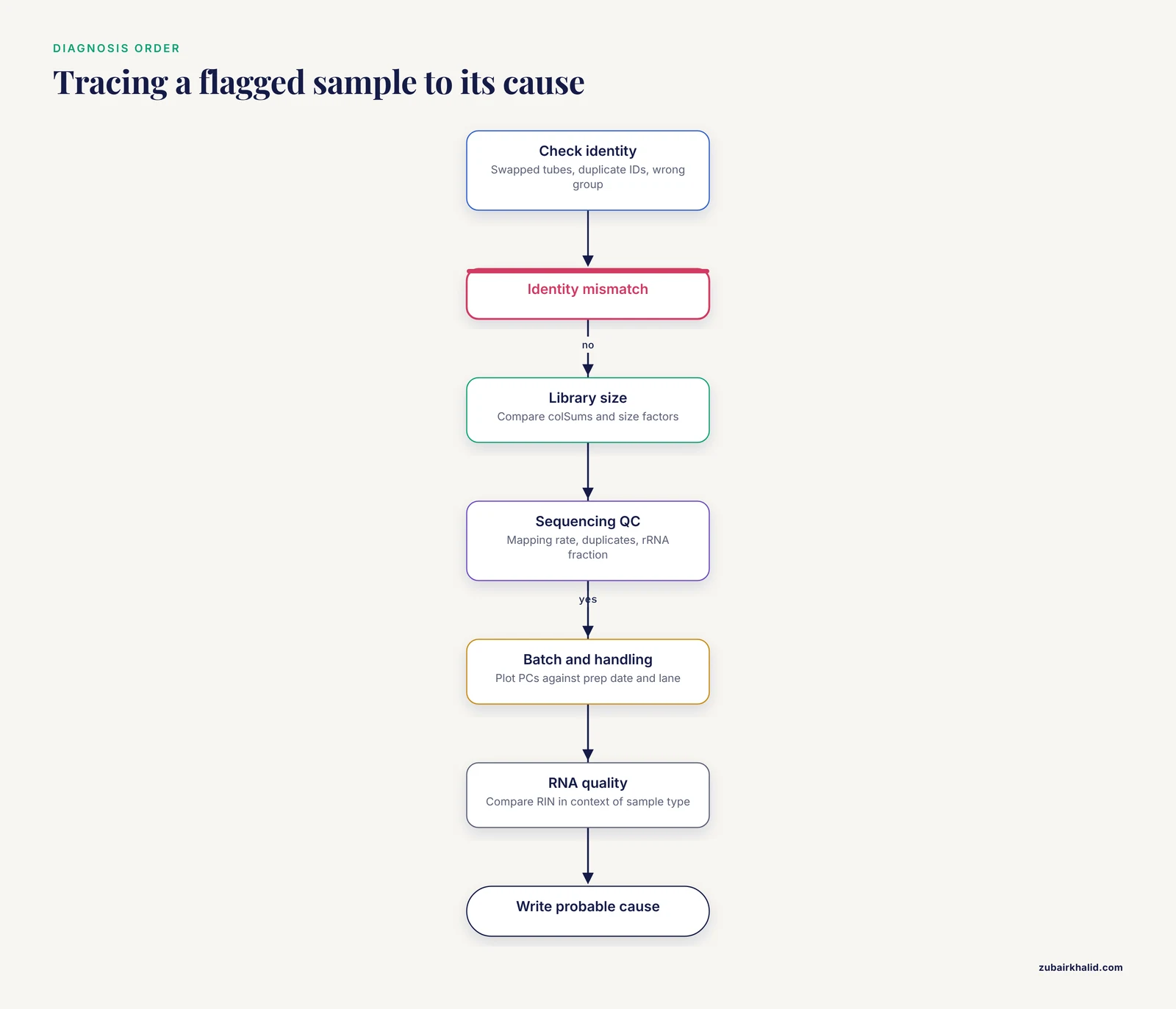
Flowchart of six checks run in order from sample identity through handling to find why a sample diverges.

A flag is not a decision. Before removing anything, interrogate why S5 diverges. Work through this checklist in order.

Metadata and identity. Check for swapped tubes, duplicated sample IDs, or a sample assigned to the wrong group. Recheck against the lab notebook and the sequencing submission sheet.
Library size and composition. Compare colSums(cts_f) across samples. A sample with a wildly different size factor, like S5 at 0.63 above, points at concentration miscalculation or skewed library composition.
Sequencing QC. Pull mapping rate, duplicate fraction, rRNA or contaminant fraction, and insertion size from your alignment logs. Low mapping rate with high rRNA content usually means degradation or failed enrichment.
Batch and handling. Plot each PC against batch variables: extraction date, library prep date, flow cell, lane. Batch effects are systematic non-biological variation, and they are common enough that automated quality-aware tools have been built specifically to detect and correct them in public RNA-seq datasets, where batch information is often underreported in publications [5].
RNA quality. Compare RIN or equivalent integrity values across samples. Interpret RIN in context rather than against a fixed universal threshold. A study of milk fat globule RNA found RIN values around 3.6 that failed the conventional RIN of at least 7 benchmark, yet RNA-seq still yielded over 52 million paired-end reads per sample that passed raw-read QC, because that sample type inherently contains low molecular-weight RNA with minimal 18S and 28S rRNA [6]. A low RIN is a red flag only when it is unusual for the sample type.
Pre-analytical handling. Some sample types are acutely sensitive to processing, storage, and transport, a point demonstrated for human blood-derived neutrophils, where the choice of collection and preservation method directly determines whether usable transcriptomes come back at all [7]. If one sample traveled farther, thawed, or sat at room temperature, that is a candidate cause you can act on in the next collection round.

Write down the most probable cause for each flagged sample before you touch the data again. This record is what turns a suspicious point on a plot into a defensible analytical decision.

Step 8. Decide: remove, correct, or keep

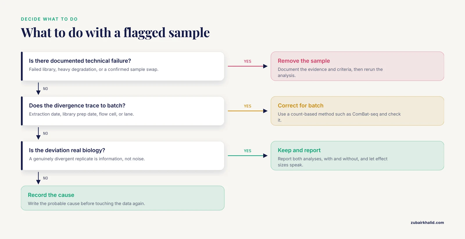
Decision path from a robust PCA flag through cause checks to removing, correcting, or keeping the sample.

You have three defensible options, and the diagnosis from Step 7 picks between them.

Remove the sample when the cause is irreversible technical failure: failed library, heavy degradation, confirmed swap. Document the removal, the evidence, and the criteria in your methods section. Then rerun the analysis. When differential expression is the next step, rerun with and without the outlier and compare results, because method behavior depends on sample size, with comparisons showing one method performing best at 3 samples per group and others such as DESeq2 performing better at 6 or 12 [8]. If your conclusion flips depending on one sample, no plot can fix that. You need more replicates.

Correct the data when the divergence traces to batch rather than sample failure. Batch correction methods built on negative binomial models, such as ComBat-seq, adjust count data while preserving the count framework, and a refined variant called ComBat-ref selects the batch with the smallest dispersion as a reference and adjusts other batches toward it, improving sensitivity and specificity on both simulated and real datasets including NASA GeneLab transcriptomic data [9]. Couple this with caution: machine-learning-based quality assessment has shown that methods for detecting unwanted variance can mistake real biological signal for a batch effect, which is exactly why quality-aware batch detection was developed, evaluated across 12 public RNA-seq datasets, and found comparable or better than a priori batch-knowledge-based correction in 11 of them [5].

Keep the sample when the divergence is real biology. The robust PCA study itself emphasizes that extreme deviation may reflect true biological differences rather than technical error [1]. A genuinely divergent biological replicate is information, not noise. Keeping it usually means reporting both analyses, with and without, and letting the effect sizes speak.

Whichever option you choose, the pipeline for the final analysis follows the standard sequence from QC through preprocessing, alignment, differential expression, and functional interpretation, with QC treated as the foundation that the rest of the analysis stands on [2].

Choosing a Detection Method

Method	Input	What it flags	Strengths	Watch out for
Visual PCA inspection	VST counts, top variable genes	Samples far from group centroid	Fast, standard, good first screen	Subjective, contaminated by the outlier itself
Robust PCA, PcaHubert	Samples by top variable genes	Score and orthogonal distance exceed robust cutoffs	Fits the majority first, resistant to masking [1]	Needs dimension reduction before use with many genes
Robust PCA, PcaGrid	Samples by top variable genes	Same distances, grid-based fitting	Best validated sensitivity and specificity in published positive-control tests [1]	Slower than classical PCA
Sample distance heatmap	Pairwise distances on VST counts	Uniformly elevated distance to all samples	Catches swapped or mislabeled libraries	No automatic threshold, judgment required
DE sensitivity analysis	Raw counts, full model	Genes whose signal depends on one sample	Measures actual impact on conclusions	Interpret with sample size in mind [8]

Use at least two methods that agree before acting. Visual PCA alone is how outliers get missed when they influence only PC3 and PC4, and visual PCA alone is also how perfectly good samples get deleted because someone expected tighter clustering than the biology allows.

Common RNA-Seq Errors You Will Hit

Bioinformatics troubleshooting goes faster when you recognize the error message instead of pasting it into a search box cold. These are the failures that show up most often between count import and PCA.

Error in estimateSizeFactorsForMatrix(counts(object)) : every gene contains at least one zero, cannot compute log geometric means

Your filter was too loose. Median-of-ratios needs genes with nonzero counts everywhere to compute geometric means. Tighten the filter or switch to estimateSizeFactors(dds, type = "poscounts").

Error in DESeqDataSetFromMatrix(...) : ncol(countData) == nrow(colData) is not TRUE

The count matrix and sample sheet disagree in dimension or order. Almost always a renamed or dropped sample. Run setdiff(colnames(cts), rownames(meta)) and setdiff(rownames(meta), colnames(cts)) to find the mismatch on both sides.

Error in checkFullRank(modelMatrix) : the model matrix is not full rank

Your design is confounded, for example every control sample run on batch A and every treated sample on batch B. No statistical correction can separate condition from batch in that design. This is a design flaw, and the fix is additional samples or a redesign, not a software flag. It connects directly to why batch effects are best addressed at the design and collection stage rather than only computationally [5].

Error in svd(x, nu = 0) : infinite or missing values in 'x'

NaNs reached the PCA. This happens when rlog runs on genes with all-zero counts or when a normalization produced division by zero. Recheck the filter, and confirm sum(is.na(assay(vsd))) returns 0 before plotting.

Robust PCA fails or returns nonsense with thousands of genes

PcaHubert and PcaGrid are multivariate methods that need a reasonable variable-to-sample ratio. Feed them the top 500 to 2,000 most variable genes after VST, samples in rows, as in Step 6. Feeding raw 20,000-gene matrices to robust PCA is a mistake of scale, not of concept [1].

Error: cannot allocate vector of size ...

Memory exhaustion, usually from running rlog on tens of thousands of genes with many samples. Use vst, which is fast and recommended for large n, or subset before transforming.

PCA looks clean but differential expression collapses

The outlier sits in PC3 or beyond. Plot PCs 1 through 4, rerun robust PCA with more components, and check the DE sensitivity comparison. Two dimensions of a six-dimensional projection cannot certify a dataset.

How to Check Your Result Is Right

Before you report or delete anything, verify along these lines.

The flagged sample is flagged by both robust methods and by the distance heatmap, not just by one view [1].
The size factor, sequencing QC, and handling metadata tell a coherent story that matches the flag. A sample that is an outlier in expression space but perfect in every QC metric deserves a second look, because it may be real biology rather than an RNA-seq error in the technical sense [1].
Removing the sample changes PCA structure the way theory predicts: PC1 variance share drops, within-group clustering tightens, and previously hidden structure may emerge. If removal changes almost nothing, consider keeping the sample and simply reporting it.
Your normalization assumption holds. If most genes are not expected to change between your conditions, median-of-ratios is appropriate. If that assumption is violated, document the alternative you used, since normalization choice propagates into every downstream result including false positive rates in differential analysis [3].
Any batch correction you applied was checked against a quality-aware assessment rather than applied blindly, because automated detection of unwanted variance can misclassify true biological signal [5].

Common Mistakes and Limitations

These are the mistakes that most often turn an outlier investigation into a retracted conclusion.

Normalizing with TPM or FPKM for PCA on the full matrix and then doing DE elsewhere. TPM and FPKM answer different questions from count-based between-sample normalization, and each normalization method rests on assumptions about how many genes move between conditions. Pick the method whose assumptions your experiment satisfies, and use one consistent pipeline from PCA through DE [3].

Deleting the outlier before diagnosing it. An unexplained deletion is indistinguishable from cherry-picking, and reviewers know it. The diagnosis chain in Step 7 exists so your exclusion criterion is evidence-based and reproducible.

Treating the PCA cluster as proof of biology. PCA clusters describe variance structure in a transformed subset of genes, nothing more. Confirm group separation with the distance matrix and, where relevant, formal tests before building conclusions on the plot.

Forgetting that outliers can be biological. The robust PCA framework was developed precisely because extreme deviation in RNA-seq can reflect either technical variation or true biological difference [1]. A treatment that genuinely reprograms one animal's transcriptome produces an outlier you should keep and report.

Blind batch correction. Applying a correction tool without batch metadata or without checking that the signal is truly unwanted variance can erase real biology. Quality-aware assessment exists for this reason and improved correction outcomes in the majority of tested public datasets when coupled with outlier removal [5].

Ignoring sample size. With three replicates per group, one sample is a third of its group and no detection method can estimate group structure reliably from the remainder. Method benchmarking shows that performance rankings themselves change between 3 and 6 or 12 samples per group [8]. Plan replicates with outlier risk in mind, including the pre-analytical handling steps that determine whether fragile sample types yield usable data at all [7].

Reading RIN as a universal gate. RIN benchmarks assume conventional tissue RNA profiles. Sample types with inherently low molecular-weight RNA or minimal ribosomal peaks can produce low RIN values and still yield millions of high-quality reads [6].

Only looking at two PCs. PC1 and PC2 summarize the largest variance directions, which the outlier may or may not occupy. Screen additional PCs and rely on the robust distances rather than the projection alone.

Where to Go Next

Once your PCA is trustworthy, several extensions follow naturally. For batch effects that survive outlier handling, negative binomial count-model corrections such as ComBat-seq and its reference-batch refinement offer a documented path to improved differential expression sensitivity [9]. If your data are single-cell rather than bulk, the same discipline applies earlier in the pipeline, and graphical tools that include a dedicated outlier-sample removal module, along with batch-effect removal and normalization modules, make the workflow accessible without custom scripting [10]. For experiments moving toward transcript-level resolution, long-read benchmarks provide guidance on when depth versus read accuracy matters most, and they recommend incorporating orthogonal data and replicate samples when rare or novel transcripts are the target [11]. And when you select genes or signatures to summarize your PCA-cleaned data, sample-wise gene set methods such as GSVA turn the expression matrix into pathway-level scores that behave well in heterogeneous populations [12], which is often the most interpretable way to present what an outlier was distorting in the first place.

Frequently Asked Questions

What cutoff defines an outlier in an RNA-seq PCA?

There is no universal numeric cutoff on a PCA plot itself. The quantitative standard is a robust distance cutoff, and the rrcov implementations flag samples whose score or orthogonal distances exceed a robust reference distribution threshold, by default near the 97.5th percentile [1]. Combine that flag with the diagnostic checklist before acting.

Can I just delete the outlier sample?

You can remove a sample when you have documented technical evidence for failure, but you should never delete based on the PCA plot alone. Diagnose first, record the criterion, and report the analysis with and without the sample when the result is close.

Should I run PCA on raw counts, TPM, or normalized counts?

Run it on variance-stabilized, filtered counts. Raw counts are dominated by total expression and highly expressed genes, and TPM or FPKM answer composition questions rather than between-sample comparison questions. The normalization method you choose should match the assumptions of your experiment [3].

How many samples do I need before PCA is meaningful?

More than two per group, and ideally enough that one bad sample cannot dominate. With three samples per group, one outlier is a third of the group and no statistical method can recover reliable group structure. Method performance itself changes between 3 and 6 or 12 samples per group in differential analysis benchmarks [8].

Is an outlier always a technical problem?

No. Extreme deviation can come from technical variation in the multi-step library protocol or from true biological differences, and both causes are real in RNA-seq data [1]. The diagnostic workflow exists to separate them, not to assume the worst.

Do I need robust PCA, or is classical PCA enough?

Classical PCA is fine for visualization but it is contaminated by the very outliers you are hunting, because it estimates the center from all points. Robust methods fit the majority first and then flag deviations, and validated implementations exist specifically for RNA-seq outlier detection [1]. Use robust methods for the decision, classical PCA for the figure.

What if the outlier appears in only one group?

Check first whether that group shares a batch, extraction date, or handling step, because a group-level batch effect can masquerade as group-specific outliers. If the design is confounded so that batch and condition cannot be separated, no correction method can recover the effect and the experiment needs additional samples [5].

Does batch correction fix outliers?

Batch correction addresses systematic differences between defined processing groups, not arbitrary single-sample failures. Quality-aware tools have made correction comparable or better than knowledge-based correction in most tested datasets, especially when coupled with outlier removal, but the outlier still needs its own diagnosis first [5].