Normalization Method RNA-seq Microarray Comparison: How to Choose

By Dr. Zubair Khalid, DVM, MS, PhD · 2026-11-11

RNA-seq normalization adjusts discrete read counts for library size and gene length so samples can be compared fairly, while microarray normalization adjusts continuous fluorescence intensities for background signal and probe behavior so arrays can be compared fairly. The rule of thumb is simple. For a standard RNA-seq differential expression experiment, use a count-based scaling method such as TMM in edgeR or the median-of-ratios method in DESeq2 after filtering low-count genes. For a microarray experiment, use RMA or an equivalent background correction plus quantile normalization pipeline. Only cross the platforms with methods built for that job, such as feature-specific quantile normalization or a multi-platform meta-analysis framework.

This guide walks through the full set of normalization method options for both platforms, weighs the pros and cons with evidence from controlled comparison studies, and gives you worked scenarios, a troubleshooting checklist, and the mistakes that most often produce a misleading result.

Why Normalization Differs Between Platforms

The two technologies measure expression in fundamentally different ways, and that difference drives every normalization choice downstream.

A microarray measures how much labeled cRNA or cDNA hybridizes to a fixed probe. The raw signal is a continuous fluorescence intensity. Sources of technical variation include background fluorescence, differences in labeling and staining efficiency, probe affinity differences, and array-to-array variation in scanning gain. Most of these effects are smooth, continuous, and well described by linear or additive models on the log scale. Methods like RMA were designed around exactly these properties.

An RNA-seq experiment counts sequencing reads assigned to each gene. The raw signal is a discrete integer count. Sources of technical variation include total sequencing depth, gene length, GC content, transcript composition, and mapper or annotation choices. Two problems dominate. First, a sample sequenced twice as deeply will show roughly twice the counts for the same gene, so library size must be corrected. Second, and less obvious, if a handful of very highly expressed genes soak up a large share of reads in one condition, the counts for every other gene are compressed, which makes naive per-million scaling unreliable. This compositional effect is the main reason simple methods fail and scaling-factor methods like TMM and median-of-ratios were developed.

A third difference matters for planning rather than for method choice. Analyses of RNA-seq count data have shown that the level of technical noise in recent RNA-seq data runs higher than in microarray data, and that the primary cause is not the counting principle itself but the overlooking of low-abundance transcripts [1]. That same analysis found that the number of biological replicates matters more than read depth for controlling this problem, because deeper sequencing does not prevent a transcript from being missed, while replicates let you estimate and absorb the variability. In microarray work, by contrast, the platform reached technical maturity years ago and its noise structure is stable and well characterized.

Side-by-Side Comparison of the Two Normalization Paradigms

Feature	RNA-seq normalization	Microarray normalization
Raw signal	Integer read counts per gene	Continuous fluorescence intensity per probe
Main problems corrected	Library size, RNA composition, gene length (for level estimates)	Background fluorescence, probe affinity, dye and labeling bias, array effects
Classic methods	Total Count, RPKM/FPKM, TPM, Upper Quartile, TMM, DESeq2 median-of-ratios, quantile	RMA, MAS5, quantile normalization, loess (within-array), variance-stabilizing transformation
Typical statistical model afterward	Negative binomial GLM (edgeR, DESeq2) or log-counts with precision weights (voom, limma)	Linear models on log2 intensities (limma)
Background correction step	Rarely explicit, handled by counting filters	Explicit and central (RMA convolution model, MAS5 mismatch subtraction)
Sensitivity to filtering low-count genes	High for several methods, documented in controlled comparisons	Lower, probes are preselected at array design
Output scale	Counts, CPM, TPM, or log2 scale	Log2-scale expression values
Best suited for	Differential expression with adequate replicates, novel transcript discovery	Well-annotated single-platform studies, reanalysis of large legacy archives

The key structural point is that microarray normalization is a preprocessing pipeline that produces the final expression matrix, while RNA-seq normalization is usually a step inside the differential expression tool itself. In edgeR, TMM factors are computed and then the negative binomial model consumes raw counts directly. In DESeq2, size factors play the same role. You generally should not extract "normalized counts" from one tool and feed them into a different statistical model, because the model assumptions are tied to the normalization scheme.

RNA-seq Normalization Method Options

Here are the main options, what each one does, and where each one breaks.

Total Count and CPM scaling

Total Count (TC) scaling divides each gene count by the total mapped reads in its sample and often scales to counts per million (CPM). It is the simplest method and requires no assumptions about which genes change between conditions.

Its weakness is composition bias. Because the denominator includes the reads assigned to every gene, a condition in which a few housekeeping-plus transcripts spike will drag down the apparent abundance of everything else. In the large Drosophila Genetic Reference Panel study that sequenced 726 individual flies and evaluated eight normalization methods with three filtering strategies, Total Count normalization did not align the data across samples and was explicitly flagged as unreliable [2]. Treat CPM as an intermediate format for filtering and visualization, not as a normalized expression estimate for statistical testing.

RPKM, FPKM, and TPM

RPKM (reads per kilobase per million mapped reads) and its paired-end version FPKM divide the gene count by both total reads and gene length. TPM (transcripts per million) first divides by gene length, then rescales so the per-sample sum is one million, which makes TPM values comparable across samples within a dataset.

These length-scaled measures answer a different question than differential expression. They estimate relative abundance per gene, which is what you want for cross-gene comparisons within a sample or for reporting expression levels. In the Drosophila evaluation, RPKM normalization again failed to align data across samples and is not appropriate as the normalization step for differential expression testing [2]. The standard practice is therefore to use raw counts plus a scaling-factor method for testing, and TPM only for descriptive reporting of expression levels.

A related but distinct use is exon-level or isoform-level analysis. One study of transposable element-derived exons across 26 RNA-seq datasets used a rescaled RPKM measure, a double-normalized quantity, to quantify exon retention rates, which shows how length-scaled measures remain useful when the unit of interest is a feature whose effective length varies [3].

Upper Quartile normalization

Upper Quartile normalization scales each sample so that the 75th percentile of the counts matches across samples. Because the scaling is based on a high percentile rather than the total, it is more robust to the composition problem than TC, though less refined than TMM. It served as the global-scaling step in newer hybrid methods evaluated on the MAQC benchmark [4].

TMM (Trimmed Mean of M-values)

TMM, implemented in edgeR through the calcNormFactors function, computes a scaling factor for each sample from the log fold changes of a trimmed set of genes that are expressed at reasonable levels and show no extreme fold changes. It directly corrects the compositional bias described above and is the default scaling approach in edgeR.

One caution comes from the Drosophila study. The Median, Quantile, and Trimmed Mean of M-values methods were sensitive to whether lowly expressed genes were removed from the dataset before normalization [2]. The practical consequence is that filtering and normalization are coupled. Filter low-count genes first, compute TMM factors on the filtered table, and report the filtering threshold in your methods section so the result is reproducible.

DESeq2 median-of-ratios

The DESeq2 median-of-ratios method forms, for each gene, the ratio of its count in a sample to the geometric mean count of that gene across all samples, then takes the median ratio per sample as the size factor. It assumes that most genes are not differentially expressed and corrects library size and composition simultaneously. It shares with TMM the sensitivity to filtering decisions and the assumption that global, symmetric shifts in expression are rare. If your experiment genuinely shifts most of the transcriptome in one direction, such as a strong global transcriptional response, both TMM and median-of-ratios can absorb real biology into their scaling factors, and spike-in-based alternatives deserve consideration.

Quantile normalization on RNA-seq

Quantile normalization forces the entire count distribution of every sample to be identical. On microarrays this is well grounded because the probe set is fixed and technical effects dominate the distribution. On RNA-seq counts, the Drosophila evaluation found that quantile normalization did not align the data across samples and behaved unpredictably when low-expressed genes were filtered [2]. Quantile normalization can still be appropriate on log-transformed, length-corrected RNA-seq values in specific cross-platform settings, which is covered in the integration section below.

A note on what "best" means

A systematic comparison framework built on measurement error models made a point that should guide every choice. Correlating a normalized RNA-seq method against a single gold standard such as qRT-PCR or microarray is statistically inadequate, because the gold standard itself carries measurement error, and a correlation coefficient tells you little about the actual quality of the normalized values [5]. Performance is better characterized by a system of error models with estimable parameters, without assuming any platform is the truth. In practice, this means the best normalization method rna-seq microarray comparison question has no universal answer. The best method is the one matched to your data structure, your filtering choices, and your downstream model.

Microarray Normalization Method Options

RMA (Robust Multiarray Averaging)

RMA is the standard pipeline for Affymetrix-type arrays. It performs three steps. Background correction adjusts raw probe intensities for optical noise using a convolution model. Quantile normalization makes the probe intensity distributions identical across arrays. Median polishing summarizes the probe-level values into one gene-level expression value per array. The output is a log2-scale expression matrix ready for linear modeling.

RMA performed well in applications beyond simple differential expression. In a comparison of gene regulatory networks inferred from Arabidopsis microarray and RNA-seq data against a gold standard of transcriptional interactions, networks built from RMA-normalized microarray data and VST-normalized RNA-seq data predicted true regulatory edges at higher rates than networks built with other normalization procedures [6].

MAS5 and one-array methods

MAS5 uses mismatch probes to estimate and subtract background on a per-array basis. It does not require a full array set, which made it historically useful for single-array analyses, but it is noisier across arrays than RMA and is rarely the first choice for multi-array studies today.

Within-array and two-color methods

Two-color arrays, where two labeled samples compete on the same slide, use within-array normalization such as loess regression to remove intensity-dependent dye bias, followed by between-array scaling. These methods are mature but apply to a platform type that has largely receded from new experiments.

Variance-stabilizing transformation

For platforms such as Illumina BeadArrays, a variance-stabilizing transformation (VST) produces values whose variance is approximately independent of the mean, which suits linear models and network inference. Its strong showing in the gene regulatory network comparison alongside RMA illustrates a broader pattern, that platform-appropriate transformations on the log or log-like scale tend to outperform raw-scale methods in downstream modeling [6].

Cross-Platform and Hybrid Normalization Methods

A growing class of methods exists specifically for the situation where microarray and RNA-seq data must be analyzed together, or where a model trained on one platform must classify data from the other.

Per-gene normalization after global scaling

Li and colleagues proposed Med-pgQ2 and UQ-pgQ2, which apply per-sample global scaling (median or upper quartile) followed by per-gene normalization so that comparisons between conditions are made at similar count levels. On the MAQC2 benchmark with two replicates, these per-gene methods achieved slightly higher area under the ROC curve than the commonly used methods they compared against (DESeq, TMM-edgeR, FPKM-CuffDiff, TC, Med, UQ, and FQ), with specificity above 85 percent and detection power above 92 percent [4]. The design insight is that global scaling handles sample-level bias while the per-gene step handles gene-level measurement differences, and the two steps are complementary rather than redundant.

Feature-specific quantile normalization (FSQN)

FSQN was built for the classifier problem. Machine learning classifiers are often trained on large microarray archives, but new samples arrive as RNA-seq. FSQN normalizes RNA-seq data so that it can be classified by models trained exclusively on DNA microarray data, reaching up to 98 percent accuracy for breast invasive carcinoma subtypes and 97 percent for colorectal cancer subtypes in the benchmark datasets, with accuracy highest when the RNA-seq dataset contains at least 25 samples [7]. The sample-size floor is a practical planning constraint. If you have fewer than about 25 RNA-seq samples, expect degraded cross-platform classification performance.

Multi-platform meta-analysis normalization

For combining multiple independent microarray and RNA-seq studies in a meta-analysis, dedicated multi-platform normalization methods adjust systematic variation so expression measures can be compared across studies while minimizing technical noise, batch effects, and platform bias [8]. This approach was applied to Affymetrix microarray and Illumina RNA-seq datasets from GEO and TCGA in cancer transcriptomics, where integrating studies is routine precisely because single-study sample sizes limit statistical power [8].

A cautionary example of why careful normalization matters in meta-analyses comes from spinal muscular atrophy, where a systematic comparative meta-analysis of six studies using both microarray and RNA-seq data found differential expression results ranging from zero to 1,655 significant genes across the selected studies, with substantial dependence on experimental settings and processing choices [9]. Divergent DEG counts like that are usually a normalization and preprocessing problem before they are a biology problem.

Learned cross-technology translation

The newest option is probabilistic machine learning frameworks that learn a unified representation of biological signal across technologies and then translate data between platforms. PXN was designed to bridge even the microarray to RNA-seq divide, preserving biological variation while removing technology-specific biases, and benchmarked better than existing normalization methods for cross-platform accuracy and differential expression power [10]. These methods require training data and validation on your own matched samples before you trust them, but they represent where the field is heading for integrating legacy microarray archives with modern RNA-seq studies.

Pros and Cons at a Glance

Method	Pros	Cons
Total Count / CPM (RNA-seq)	Simple, assumption-free, fast for filtering	Fails to align samples under composition bias [2]
RPKM/FPKM (RNA-seq)	Length-corrected levels, intuitive	Not aligned across samples for DE testing [2]
TPM (RNA-seq)	Sample-comparable abundance estimates	Descriptive only, not for DE testing
Upper Quartile (RNA-seq)	More robust than TC, simple	Crude relative to TMM and median-of-ratios
TMM (RNA-seq)	Corrects composition bias, edgeR default	Sensitive to low-expression filtering choices [2], assumes most genes unchanged
Median-of-ratios (RNA-seq)	Robust, DESeq2 default, well understood	Same filtering sensitivity and no-global-shift assumption [2]
Quantile on raw counts (RNA-seq)	None demonstrated in controlled tests	Did not align samples [2]
RMA (microarray)	Mature, excellent bias control, log2 output	Platform-specific, no probe flexibility for novel transcripts
MAS5 (microarray)	Works on single arrays	Noisier than RMA in multi-array studies
VST (microarray/RNA-seq)	Stabilizes variance for modeling	Extra transformation step to justify and report
Med-pgQ2 / UQ-pgQ2 (hybrid)	High specificity and power on MAQC2 with 2 replicates [4]	Newer, requires benchmarking in your own context
FSQN (cross-platform)	Enables microarray-trained classifiers on RNA-seq [7]	Needs roughly 25 or more RNA-seq samples
Multi-platform meta normalization	Unlocks pooled power across GEO and TCGA studies [8]	Requires matched feature mapping and careful batch diagnostics
PXN (learned translation)	Cross-platform accuracy beyond classical methods [10]	Needs training data, validation on matched samples

The Criteria That Decide Real Choices

What question are you answering?

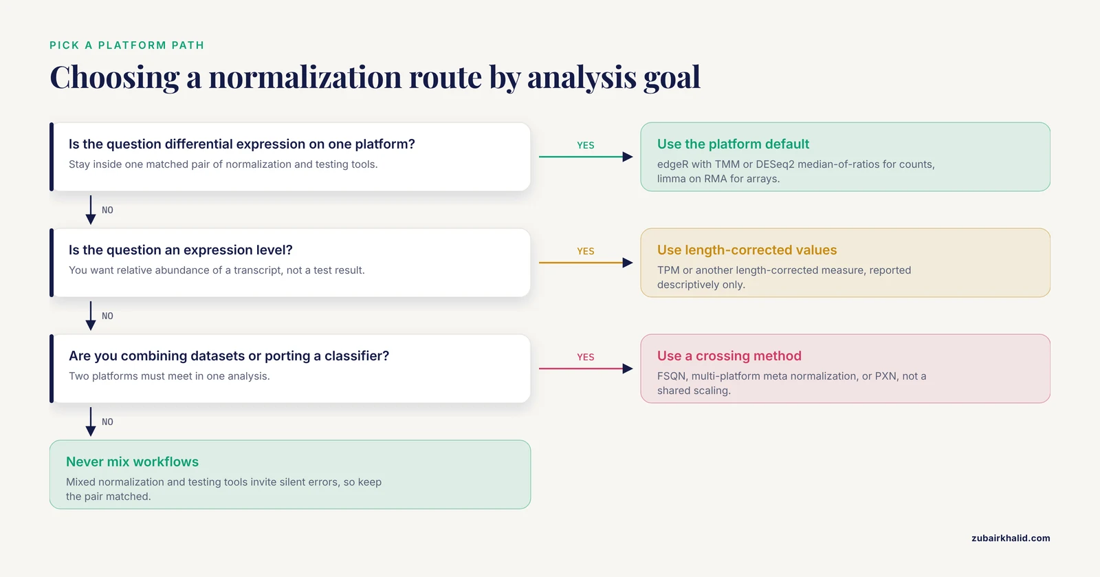
Decision path asking whether the question is differential expression, an expression level, or an integration, and naming the matching method family.

If the question is differential expression within one experiment on one platform, stay within a single well-matched pair of normalization and testing tools. edgeR plus TMM, or DESeq2 plus median-of-ratios, for RNA-seq counts. limma on RMA-normalized values for microarrays. Mixed workflows invite silent errors.

If the question is an expression level (how abundant is this transcript), TPM or a length-corrected measure is appropriate, and this is also where cross-platform level comparisons are most often attempted.

If the question is integrative (combine datasets, port a classifier, run a meta-analysis), use methods designed for the crossing, not a shared normalization applied naively.

How many replicates do you have?

Replicate number dominates power in RNA-seq. The Drosophila study with eight biological replicates per condition concluded that the normalization method, the distributional assumption, and the replicate number were the most critical considerations for RNA-seq analysis, an observation consistent with earlier RNA-seq and microarray comparisons [2]. Low-replicate designs change the calculus. The MAQC2 benchmark work showed that per-gene hybrid methods can hold specificity and power even with only two replicates [4], but two replicates cannot estimate variance robustly in a negative binomial model, so low-replicate designs deserve either benchmarked methods or conservative interpretation.

How much do you trust each platform?

Controlled head-to-head studies with matched samples give a realistic picture. In a comparison on matched Jurkat T cell samples run on both an Affymetrix HTA2.0 microarray and paired-end RNA-seq, overall agreement between the platforms was high, with better sensitivity from the RNA-seq analysis [11]. In dermal mesenchymal stem cells, both platforms identified 23 differentially expressed genes in common, with concordant direction for 14 of 23, and validation against real-time PCR showed an 83.3 percent coincidence rate for RNA-seq versus 37.5 percent for microarray, a significant difference favoring RNA-seq, which also revealed more than 2,300 novel transcription tags absent from array probes [12].

Platform behavior differs by design, however. In a dose-response toxicology experiment in rats exposed to bromobenzene across five doses for 13 weeks, with both platforms measured on the same liver samples and multiple normalization methods evaluated for each, fold-change values correlated highly between technologies while log p-values correlated less well, RNA-seq detected fewer significant genes at lower doses but more by fold change, overlap in genes significant by both criteria was roughly 30 to 40 percent, and qRT-PCR confirmed genes unique to either platform at high rates when both fold change and p value were considered [13]. The same study showed that with about 5 million reads, randomly sampled RNA-seq data detected roughly the same number of differentially expressed genes as microarrays [13], a useful planning number for budget-limited designs.

Statistical framework matters as much as normalization

Platform comparisons are sensitive to the statistical approach, not only the normalization. A recent matched-sample study in whole blood from 35 participants analyzed both microarray and RNA-seq with non-parametric Mann-Whitney U tests and found a median Pearson correlation of 0.76 in gene expression profiles, with RNA-seq identifying 2,395 differentially expressed genes against 427 on microarray and 223 genes shared, while pathway analysis found 205 perturbed pathways from RNA-seq, 47 from microarray, and 30 shared [14]. The authors concluded the two technologies give highly concordant results when analyzed with consistent statistical methods and can be used complementarily [14]. A separate matched-sample study in rectal cancer and Burkitt lymphoma specimens compared four RNA-seq pipelines (STAR/HTSeq-Count/edgeR, STAR/RSEM/edgeR, Sailfish/edgeR, and TopHat2/Cufflinks/CuffDiff) against microarray preprocessing and found gene expression correlations that were moderately worse for patient tissue (Spearman 0.67 to 0.69) than for the cell line (0.87 to 0.88), a gap that sample complexity and mapping rates helped explain [15].

The lesson for normalization choice is that a pipeline decision is a joint decision. Normalization, transformation, and the statistical model interact, and a comparison run with inconsistent models across platforms will exaggerate platform differences that better methods would close.

Worked Scenarios

Scenario 1. Standard RNA-seq differential expression, two groups, six versus six

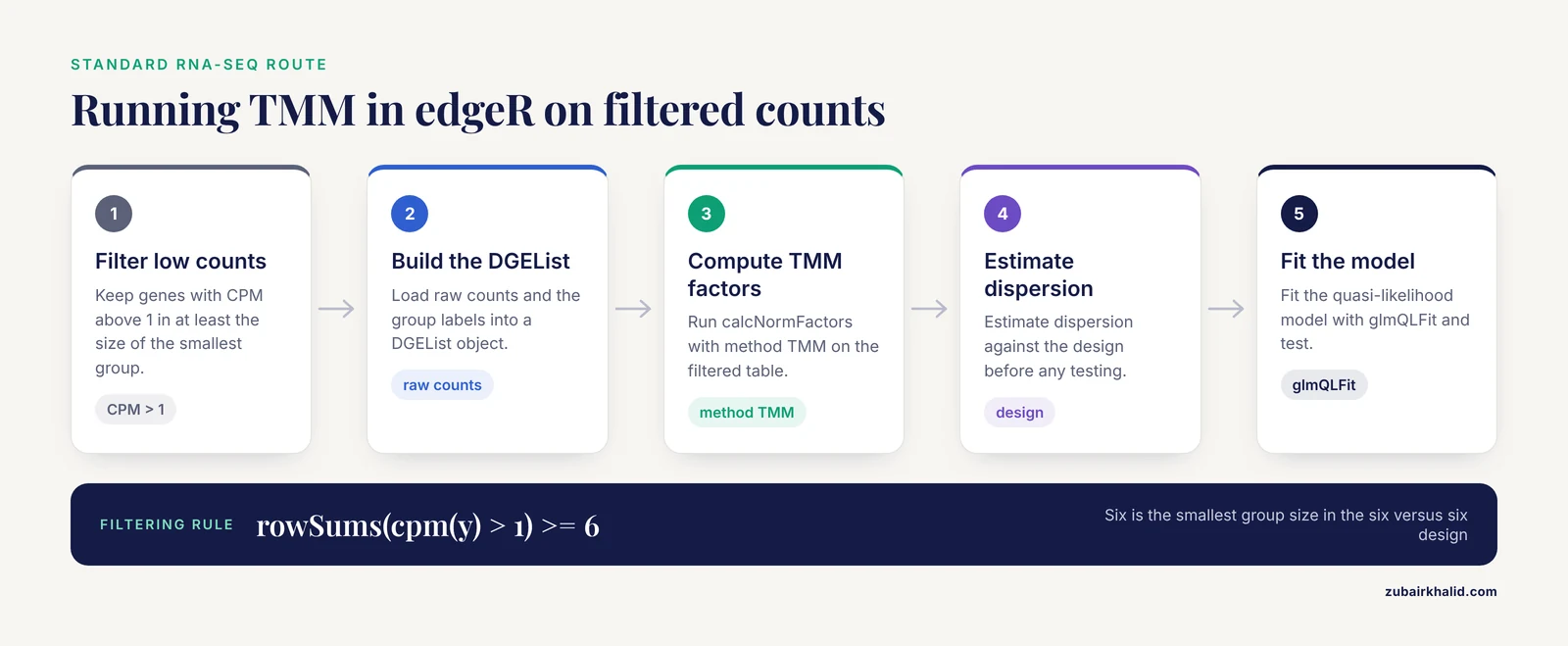
Five-step RNA-seq pipeline: filter low counts by CPM, build the DGEList, compute TMM factors, estimate dispersion, then fit the model.

Filter genes with very low counts first (for example, keep genes with CPM above 1 in at least the size of the smallest group). Then run edgeR with TMM:

library(edgeR)
y <- DGEList(counts = counts, group = group)
keep <- rowSums(cpm(y) > 1) >= 6
y <- y[keep, , keep.lib.sizes = FALSE]
y <- calcNormFactors(y, method = "TMM")
y <- estimateDisp(y, design)
fit <- glmQLFit(y, design)

The same data in DESeq2 would use its median-of-ratios size factors automatically inside DESeqDataSetFromMatrix. Either is defensible. Report the filtering rule, the normalization method, and the model. Do not report TPM values alongside DE test results as though they were the normalized values used for testing.

Scenario 2. Reanalysis of a GEO microarray dataset

Download raw CEL files if available, not processed values, because you need to control normalization. Apply RMA through the affy or oligo packages:

library(oligo)
eset <- rma(celFiles)

Then use limma on the log2 expression matrix. If only processed values exist, check whether they are already log2-scale and whether quantile normalization was applied, and document whatever you inherit rather than re-normalizing blindly.

Scenario 3. Combining TCGA RNA-seq with GEO microarray cohorts for a meta-analysis

Do not concatenate the matrices. Process each platform with its native normalization, restrict to shared genes, and combine at the level of gene-level statistics or with a multi-platform normalization method designed to remove platform bias while preserving biological signal [8]. Validate with a known positive control, such as a subtype marker expected to separate groups in both cohorts. If you need sample-level integration for classification, FSQN is a benchmarked option, provided you have at least roughly 25 RNA-seq samples [7].

Scenario 4. Dose-response toxicology with both platforms

Follow the design of the bromobenzene study. Evaluate more than one normalization method per platform rather than assuming a single default, expect fold changes to agree better than p-values, and interpret concordance using both criteria together, since the overlap between platforms reached only about 30 to 40 percent when genes had to be significant by p-value and fold change simultaneously [13]. If your budget limits sequencing depth, remember the roughly 5 million read benchmark for DEG counts comparable to microarrays in that system [13].

Scenario 5. Applying a microarray-trained molecular subtype classifier to new RNA-seq samples

Use FSQN or a learned translation framework such as PXN rather than ad hoc scaling [10], [7]. Check accuracy on a subset with known labels before committing to the full cohort, and respect the sample-size floor documented for FSQN [7].

Common Mix-Ups

These are the errors seen most often in real analyses and review cycles.

Using TPM or RPKM for differential testing. Length-corrected values are abundance estimates. Differential testing belongs on raw counts inside edgeR, DESeq2, or limma-voom. The Drosophila evaluation demonstrated directly that RPKM normalization did not align RNA-seq data across samples [2].

Normalizing before filtering on raw data. For methods that use medians or trimmed means, the filtering step changes the normalization factors. Median, Quantile, and TMM normalization were all sensitive to removal of low-expressed genes in controlled evaluation [2]. Filter first, normalize second, and keep the order fixed across all comparisons.

Running quantile normalization on raw RNA-seq counts. Quantile normalization was built for fixed probe sets on continuous intensities. Applied to raw counts, it failed to align samples in evaluation [2]. Its legitimate RNA-seq uses are on transformed values within defined cross-platform frameworks such as FSQN [7].

Assuming RMA-normalized microarray values and TPM values are on comparable scales. They are not. Directly plotting or correlating them without mapping and rescaling produces correlations that describe platform artifacts more than biology.

Ignoring annotation version. The choice of gene annotation changes RNA-seq quantification itself, before any normalization. Using the SEQC benchmark dataset with more than 800 real-time PCR validated genes and known titration ratios, RefSeq gene annotation models produced better quantification accuracy than Ensembl models, and recent expansion of the RefSeq annotation reduced its accuracy, meaning annotation updates can shift quantification in either direction [16]. A cross-platform comparison built on mismatched annotation will show disagreement that normalization cannot fix.

Trusting a single correlation with a gold standard. As the measurement error model work showed, qRT-PCR and microarray references carry their own error, and correlation-based validation understates method differences [5]. Whenever possible, validate with more than one reference and with error models rather than a single correlation coefficient.

Feeding normalized counts from one tool into another tool's model. TMM factors and DESeq2 size factors are paired with their respective statistical models. Mixing them breaks the variance model silently.

Common Mistakes and Limitations

Beyond the method mix-ups, several troubleshooting patterns recur in RNA-seq and cross-platform work. These are the practical checks that catch an rna seq error before it becomes a wrong conclusion.

Check distribution alignment before anything else. Plot per-sample density curves of log2 values and a boxplot of normalized values. In RNA-seq, samples whose count distributions fail to overlap after normalization usually have a library problem or a swap, not a normalization problem. In microarrays, RMA's quantile step will make distributions look identical even when one array is bad, so also inspect RLE (relative log expression) plots and NUSE (normalized unscaled standard error) values for array-level quality problems.

Watch for composition artifacts in RNA-seq. If a small number of genes absorb a large share of reads in one condition, per-million scaling will smear that effect across the whole table. TMM and median-of-ratios exist precisely for this. If you suspect a genuine global shift rather than a technical artifact, examine the distribution of all log fold changes, not just the significant ones.

Treat read depth and replicate number as separate levers. Increasing depth raises sensitivity for abundant transcripts but does not prevent low-abundance transcripts from being overlooked, while replicates directly improve variance estimation [1]. A common planning mistake is spending the entire budget on depth and leaving one replicate per condition.

Account for platform dynamic range honestly. RNA-seq provides a wider dynamic range and detects transcripts absent from array probe sets, which is why the mesenchymal stem cell study found over 2,300 novel transcription tags invisible to the array [12]. A differential gene list that is larger on RNA-seq is not automatically an error, but it is also not automatically a better list. qRT-PCR validation of platform-specific calls is the decisive test, and it favored RNA-seq substantially in that head-to-head comparison [12].

Expect pipeline effects upstream of normalization. In the rectal cancer and Burkitt lymphoma pipeline comparison, mapping rates ranged from 98.98 percent for STAR down to 54.44 percent for Sailfish on the patient dataset, and those upstream differences propagated into expression correlations [15]. A normalization method cannot rescue a quantification step that lost nearly half the reads.

In inflammatory and clinical signatures, verify the platform on your tissue type. In FFPE renal cell carcinoma specimens, the NanoString nCounter system and targeted RNA-seq both showed high technical reproducibility with Pearson coefficients of at least 0.96, but RNA-seq displayed larger signal intensity while nCounter showed higher inter-sample variability [17]. Platform behavior is tissue- and sample-quality-specific, so benchmarks from fresh frozen samples do not automatically transfer to FFPE.

Meta-analyses amplify processing differences. The spinal muscular atrophy meta-analysis across six studies found DEG counts ranging from zero to 1,655 depending on the study, a spread that reflects experimental settings and analysis choices as much as biology [9]. When combining platforms, document every preprocessing decision per study and run sensitivity analyses under alternative normalization schemes.

The core limitation. No normalization method creates information that the design lacks. Method choice, filtering, statistical model, and annotation interact, so the strongest protection is a small validation set: a handful of genes checked by qRT-PCR, a pathway expected to move, and a PCA plot that clusters by biology rather than by batch or platform. Individual datasets still deserve expert review of these diagnostics before any biological conclusion is drawn.

Frequently Asked Questions

Which is the best normalization method for RNA-seq differential expression?

For most two-group or factorial RNA-seq experiments, TMM in edgeR or the median-of-ratios method in DESeq2, applied to filtered raw counts, is the defensible default. Controlled evaluations found that Total Count, Quantile, and RPKM failed to align RNA-seq data across samples, while the recommended scaling methods were sensitive to low-expression filtering, so filter first and report the threshold [2]. If you have two replicates, hybrid per-gene methods benchmarked on MAQC2 are an option worth testing [4].

Can I normalize RNA-seq and microarray data together in one analysis?

Not with a single shared normalization step. Process each platform with its native method first, then combine through a cross-platform framework. Benchmark options include FSQN for microarray-trained classifiers on RNA-seq data [7], multi-platform normalization for meta-analyses of GEO and TCGA cohorts [8], and learned translation frameworks such as PXN built specifically to bridge the microarray to RNA-seq divide [10].

Should I use TPM or TMM for differential expression?

Use TMM, or a DESeq2 size factor, for differential expression. Use TPM only to report expression levels. TPM corrects for gene length and library composition but does not provide the statistical scaling that count-based models require, and RPKM-style measures were shown not to align data across samples for testing purposes [2].

Does quantile normalization work for RNA-seq?

Not on raw counts. In a controlled eight-method evaluation, quantile normalization did not align RNA-seq samples and behaved inconsistently with respect to gene filtering [2]. Its valid uses on RNA-seq are within cross-platform frameworks, where feature-specific quantile normalization is applied specifically so RNA-seq data can be compared against microarray references [7].

How many reads do I need to match microarray-level gene detection?

In a matched dose-response study in rat liver, randomly sampled RNA-seq data detected roughly the same number of differentially expressed genes as microarrays at about 5 million reads [13]. Treat that as a system-specific planning figure, not a universal minimum, and remember that biological replicates do more for reliability than added depth [1].

Why do RNA-seq and microarray experiments give different gene lists?

Different dynamic ranges, probe coverage, noise structure, and statistical frameworks all contribute. On matched samples, studies have reported high overall agreement with better sensitivity for RNA-seq [11], RNA-seq advantage in qRT-PCR validation (83.3 versus 37.5 percent coincidence with real-time PCR) [12], and much larger differential gene counts on RNA-seq under consistent statistical methods, with only a fraction of genes shared [14]. Divergent lists usually reflect real platform differences in sensitivity and the normalization and model choices you made, not a failure of either technology.