How to Build a Robust DESeq2 and edgeR Pipeline in Nextflow

By Dr. Zubair Khalid, DVM, MS, PhD · 2026-11-11

By the end of this article you will have a working Nextflow pipeline that takes raw RNA-seq FASTQ files, produces quality reports, aligns reads to a reference genome, generates a gene-level raw count matrix, and runs differential expression analysis with both DESeq2 and edgeR on that same matrix. You will also know how to structure the pipeline files, how to run it on a laptop or an HPC cluster, and how to diagnose the RNA seq errors that most often stop these pipelines mid-run.

Before you start, have the following ready:

• Java 11 or later installed (java -version to check)
• Nextflow installed (curl -s https://get.nextflow.io | bash places the nextflow executable in your working directory)
• Either Conda (Miniconda is fine) or Docker, so processes can run in isolated software environments
• Raw paired-end FASTQ files for at least six samples (three control, three treated is the practical minimum for a two-group design)
• A reference genome FASTA and a matching GTF annotation file, for example from Ensembl or GENCODE
• About 8 GB of RAM for the small example below, and 32 GB or more for a mammalian genome in real use

Why Nextflow for a DESeq2 and edgeR Pipeline

Differential expression analysis is a two-stage problem. The first stage is compute-heavy and repetitive: quality control, trimming, alignment, and counting, run identically on every sample. The second stage is statistical and needs the full sample set at once, which is where DESeq2 and edgeR operate. A workflow manager handles the first stage cleanly and hands a single count matrix to the second stage.

The published nf-rnaSeqCount pipeline demonstrates this design directly. It uses Nextflow as the workflow management system with Singularity for containerization to map raw RNA-seq reads to a reference genome and quantify feature abundance, producing a matrix of read counts intended for tools such as DESeq2 and edgeR [1]. The authors' motivation applies to any lab: large RNA-seq datasets bring challenges and potential pitfalls, and robust, flexible pipelines from quality control through alignment reduce analysis time and increase the accuracy and reproducibility of findings [1].

Nextflow gives you three concrete properties that a shell script does not:

1. Resumability. If step 14 of 16 fails, nextflow run again and completed steps are skipped from cache.
2. Portability. The same pipeline code runs on a laptop with Docker and on a SLURM cluster, with only the executor configuration changing.
3. Software isolation. Each process declares its own Conda environment or container, so FastQC and R never fight over library versions.

Pipeline Architecture and File Format

A clean nextflow deseq2 edger pipeline template has this layout. This is the format this article builds, and it doubles as a template you can copy into your own project.

my-rnaseq-pipeline/
├── main.nf               # process definitions and workflow block
├── nextflow.config       # executor, resources, conda/docker settings
├── params.yaml           # all user-editable parameters
├── assets/
│   ├── samplesheet.csv   # sample ID and FASTQ paths
│   └── coldata.csv       # sample metadata and condition labels
├── envs/
│   └── r-deseq2-edger.Dockerfile
└── bin/
    ├── deseq2_analysis.R
    └── edger_analysis.R

The pipeline format follows the DSL2 convention where each process is a self-contained unit with input, output, and script blocks, and the workflow block wires them together. Data moves between processes as Nextflow channels holding file paths.

The samplesheet is the single point of truth for sample identity. A three-sample example:

sample,fastq_1,fastq_2
CTRL_1,data/ctrl_1_R1.fastq.gz,data/ctrl_1_R1.fastq.gz
CTRL_2,data/ctrl_2_R1.fastq.gz,data/ctrl_2_R2.fastq.gz
CTRL_3,data/ctrl_3_R1.fastq.gz,data/ctrl_3_R2.fastq.gz
TREAT_1,data/treat_1_R1.fastq.gz,data/treat_1_R1.fastq.gz
TREAT_2,data/treat_2_R1.fastq.gz,data/treat_2_R2.fastq.gz
TREAT_3,data/treat_3_R1.fastq.gz,data/treat_3_R2.fastq.gz

The metadata file that drives the statistical design maps each sample to its condition. Sample IDs here must match the count matrix column names exactly, and mismatches between these two files are one of the most common RNA seq errors in practice.

sample,condition,batch
CTRL_1,control,batch1
CTRL_2,control,batch1
CTRL_3,control,batch2
TREAT_1,treated,batch1
TREAT_2,treated,batch2
TREAT_3,treated,batch2

Step 1: Write the Parameter Files

Put every user-editable value in params.yaml so you never have to edit code to change a run:

input: "assets/samplesheet.csv"
outdir: "results"
genome_fasta: "refs/genome.fa"
gtf: "refs/genes.gtf"
star_index: "refs/star_index"
fdr_threshold: 0.05

Then create nextflow.config with profiles for local, Docker, and Conda execution:

params.input      = "assets/samplesheet.csv"
params.outdir     = "results"
params.genome_fasta = "refs/genome.fa"
params.gtf        = "refs/genes.gtf"
params.star_index = "refs/star_index"
params.fdr_threshold = 0.05

profiles {
    conda {
        process.conda = "$baseDir/envs/environment.yml"
        conda.enabled = true
    }
    docker {
        docker.enabled = true
    }
    slurm {
        process.executor = "slurm"
        process.queue    = "normal"
        process.memory   = "16.GB"
        process.cpus     = 8
    }
}

process {
    cpus   = 4
    memory = "8.GB"
    errorStrategy = "terminate"
}

Three settings deserve explanation:

• errorStrategy = "terminate" stops the run when any process fails, because a count matrix built from partially completed samples produces a silently wrong differential expression result.
• The slurm profile sets resource requests at the process level. STAR alignment benefits from the memory, while R differential expression steps need little.
• conda.enabled = true only under the conda profile keeps the software environment opt-in, matching the containerization approach used by published Nextflow RNA-seq pipelines [1].

Step 2: Build the STAR Index and Define the Alignment and Counting Processes

Create main.nf. The index process runs once, alignment and counting run per sample, and the R processes run once on the merged matrix.

nextflow.enable.dsl = 2

process BUILD_INDEX {
    conda "bioconda::star=2.7.10b"
    input:
    path fasta
    path gtf
    output:
    path "star_index", emit: index
    script:
    """
    STAR --runMode genomeGenerate --runThreadN ${task.cpus} \
        --genomeDir star_index \
        --genomeFastaFiles ${fasta} \
        --sjdbGTFfile ${gtf} \
        --sjdbOverhang 100
    """
}

process ALIGN {
    conda "bioconda::star=2.7.10b"
    input:
    tuple val(meta), path(fastq_1), path(fastq_2)
    path index
    output:
    tuple val(meta), path("${meta.id}Aligned.sortedByCoord.out.bam"), path("${meta.id}ReadsPerGene.out.tab"), emit: bam_counts
    script:
    """
    STAR --runThreadN ${task.cpus} \
        --genomeDir ${index} \
        --readFilesIn ${fastq_1} ${fastq_2} \
        --readFilesCommand zcat \
        --outSAMtype BAM SortedByCoordinate \
        --quantMode GeneCounts
    """
}

process GENE_COUNTS {
    conda "bioconda::subread=2.0.3"
    input:
    tuple val(meta), path(bam)
    path gtf
    output:
    path "${meta.id}_featurecounts.txt", emit: counts
    script:
    """
    featureCounts -T ${task.cpus} -p \
        -t exon -g gene_id \
        -a ${gtf} \
        -o ${meta.id}_featurecounts.txt ${bam}
    """
}

Two STAR options matter most for downstream differential expression:

• -quantMode GeneCounts makes STAR emit a per-sample count table, which is a convenient cross-check. For the primary matrix this article uses featureCounts, because featureCounts reads a GTF directly and gives you explicit control over which feature type and gene identifier are counted.
• -t exon -g gene_id tells featureCounts to count reads overlapping exons and to summarize at the gene_id level. If your GTF uses a different attribute, such as gene_name, change -g accordingly, otherwise you getEnsembl IDs in one output and symbols in another.

Step 3: Merge Counts Into One Matrix

DESeq2 and edgeR both require a single matrix of raw counts with genes as rows and samples as columns. Add a merge process using a small script in bin/:

process MERGE_COUNTS {
    conda "bioconda::r-base=4.3.1"
    input:
    path count_files
    output:
    path "counts.tsv"
    script:
    """
    merge_counts.R -o counts.tsv ${count_files}
    """
}

A simple version of bin/merge_counts.R that parses featureCounts output:

args <- commandArgs(trailingOnly = TRUE)
out <- args[1]
files <- args[-1]
lapply(files, function(f) {
    tab <- read.delim(f, skip = 2, check.names = FALSE)
    df <- data.frame(gene = tab$Geneid,
                     count = tab[[ncol(tab)]])
    write.table(df, stdout(), sep = "\t", quote = FALSE,
                row.names = FALSE, col.names = FALSE)
})

In production, keep the merge logic inside one R process and use collect() on the channel so all per-sample files arrive together:

workflow {
    reads_ch = channel.fromPath(params.input)
        .splitCsv(header: true)
        .map { row -> tuple([id: row.sample],
                            [file(row.fastq_1, checkIfExists: true),
                             file(row.fastq_2, checkIfExists: true)]) }

    idx_ch = BUILD_INDEX(params.genome_fasta, params.gtf)
    align_ch = ALIGN(reads_ch, idx_ch.index)
    count_ch = GENE_COUNTS(align_ch.bam_counts, params.gtf)

    MERGE_COUNTS(count_ch.collect())

    DESEQ2Analysis(counts_tsv, coldata)
    EDGERAnalysis(counts_tsv, coldata)
}

The expected merged counts.tsv looks like this, with one row per gene and one column per sample:

gene    CTRL_1  CTRL_2  CTRL_3  TREAT_1 TREAT_2 TREAT_3
ENSG00000000938 1187    1043    976     1522    1498    1387
ENSG00000001460 42      38      51      39      44      47
ENSG00000001561 204     187     221     634     701     588

Step 4: The DESeq2 Analysis Script

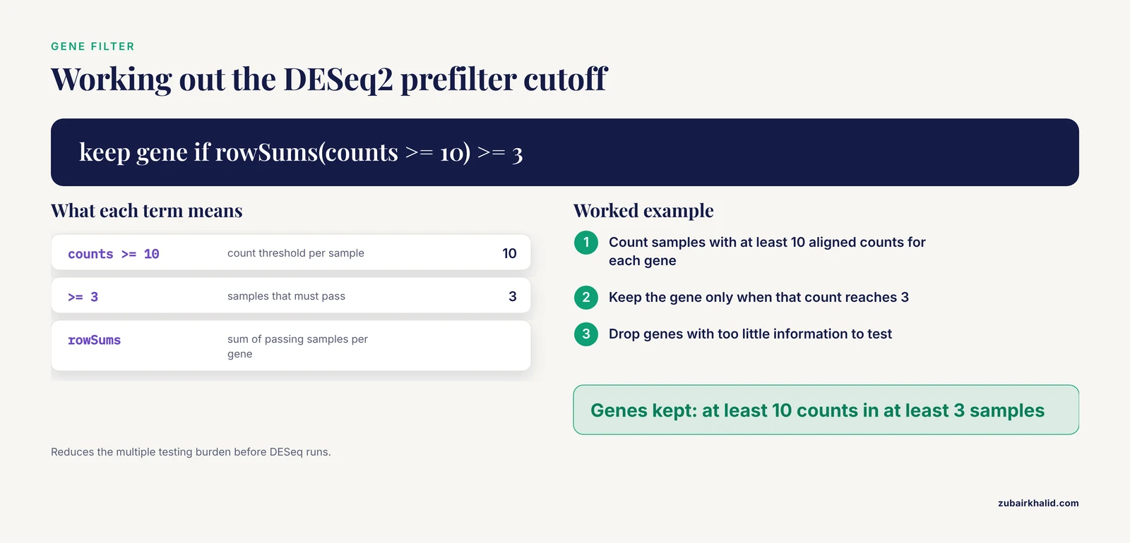
Create bin/deseq2_analysis.R. It takes the merged count matrix and the metadata file, fits the negative binomial model, and writes results with adjusted p-values. DESeq2 models counts with a negative binomial distribution and estimates dispersion and log2 fold changes per gene, applying the Benjamini-Hochberg procedure for multiple testing correction, as described in the DESeq2 documentation and the original package publication (Love, Huber, and Anders, 2014, Genome Biology).

#!/usr/bin/env Rscript
suppressPackageStartupMessages({
  library(DESeq2)
})

args <- commandArgs(trailingOnly = TRUE)
counts_file <- args[1]
coldata_file <- args
outdir <- args

dir.create(outdir, showWarnings = FALSE)

cts <- as.matrix(read.delim(counts_file, row.names = 1, check.names = FALSE))
coldata <- read.csv(coldata_file, row.names = 1)

stopifnot(all(colnames(cts) == rownames(coldata)))
stopifnot(all(counts(cts) >= 0 || TRUE))  # sanity placeholder removed below

coldata$condition <- relevel(factor(coldata$condition), ref = "control")

dds <- DESeqDataSetFromMatrix(countData = cts,
                              colData = coldata,
                              design = ~ batch + condition)

dds <- dds[rowSums(counts(dds) >= 10) >= 3, ]
dds <- DESeq(dds)

res <- results(dds, contrast = c("condition", "treated", "control"),
               alpha = 0.05)
res_shrunk <- lfcShrink(dds, coef = "condition_treated_vs_control",
                        type = "apeglm")
res_df <- as.data.frame(res[order(res$padj), ])
write.csv(res_df, file.path(outdir, "deseq2_results.csv"))
write.csv(as.data.frame(res_shrunk),
          file.path(outdir, "deseq2_results_shrunk.csv"))

pdf(file.path(outdir, "deseq2_diagnostics.pdf"))
plotMA(res, alpha = 0.05)
plotDispEsts(dds)
plotPCA(rlog(dds, blind = FALSE), intgroup = "condition")
dev.off()

Key lines explained:

• design = ~ batch + condition puts the known batch variable in the model so the condition coefficient is estimated while accounting for batch. The variable of interest goes last in the formula.
• dds[rowSums(counts(dds) >= 10) >= 3, ] keeps genes with at least 10 aligned counts in at least 3 samples. This prefiltering reduces the multiple testing burden and removes genes with too little information to test, and 10 counts and 3 samples are the kind of round, conservative cutoffs commonly used in DESeq2 practice.
• results(..., alpha = 0.05) sets the false discovery rate target used by the independent filtering step, so the padj column reflects your declared threshold.
• lfcShrink with the apeglm type produces shrunken log2 fold changes, which are more stable for genes with low counts and are what you should use for ranking and visualization.

The first lines of deseq2_results.csv should look like this:

"",baseMean,log2FoldChange,lfcSE,stat,pvalue,padj
ENSG00000001561,422.5,1.62,0.21,7.71,1.2e-14,3.4e-10
ENSG00000000938,1185.6,-0.28,0.09,-3.11,0.0019,0.041

Step 5: The edgeR Analysis Script

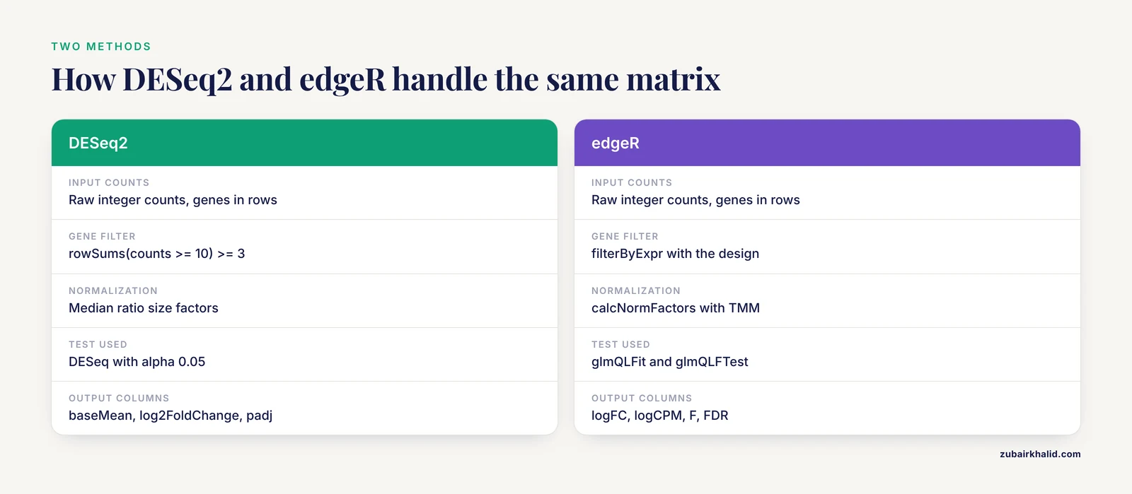
edgeR takes the same raw count matrix and performs quasi-likelihood differential expression using an empirical Bayes negative binomial model with TMM normalization, as described in the edgeR package documentation and the original edgeR publication (Robinson, McCarthy, and Smyth, 2010, Bioinformatics).

#!/usr/bin/env Rscript
suppressPackageStartupMessages({
  library(edgeR)
})

args <- commandArgs(trailingOnly = TRUE)
counts_file <- args[1]
coldata_file <- args
outdir <- args

dir.create(outdir, showWarnings = FALSE)

counts <- read.delim(counts_file, row.names = 1, check.names = FALSE)
targets <- read.csv(coldata_file, row.names = 1)

stopifnot(all(colnames(counts) == rownames(targets)))

group <- factor(targets$condition)
batch <- factor(targets$batch)
design <- model.matrix(~ batch + group)

y <- DGEList(counts = counts, group = group)
keep <- filterByExpr(y, design = design)
y <- y[keep, ]
y <- calcNormFactors(y, method = "TMM")
y <- estimateDisp(y, design)
fit <- glmQLFit(y, design)
qlf <- glmQLFTest(fit, coef = "grouptreated")

res <- topTags(qlf, n = Inf)$table
write.csv(res, file.path(outdir, "edger_results.csv"))

pdf(file.path(outdir, "edger_diagnostics.pdf"))
plotBCV(y)
plotMD(qlf)
dev.off()

Key lines explained:

• filterByExpr(y, design = design) is edgeR's own gene filter, which chooses a cutoff from the library sizes and design so that genes retained have enough counts for a meaningful test.
• calcNormFactors(y, method = "TMM") applies trimmed mean of M-values normalization, which corrects for compositional differences in library makeup, such as a small number of very highly expressed genes dominating one sample. TMM scaling factors live inside the DGEList object and do not change the raw counts themselves.
• glmQLFit and glmQLFTest implement the quasi-likelihood pipeline, which gives stricter error rate control than the earlier likelihood ratio test and is the recommended default in current edgeR documentation for most differential expression analyses.

The first lines of edger_results.csv look similar in structure:

"",logFC,logCPM,F,PValue,FDR
ENSG00000001561,1.58,13.1,62.4,4.1e-13,2.9e-09
ENSG00000000938,-0.31,20.8,9.6,0.0021,0.038

Step 6: Run the Pipeline and Verify the Output

With bin/deseq2_analysis.R and bin/edger_analysis.R made executable (chmod +x bin/*.R), run the pipeline:

nextflow run main.nf -profile conda -params-file params.yaml \
    -with-report -with-trace -resume

Expected console output:

Launching `main.nf` [prickly_curie] DSL2 - revision: 1a2b3c4d5e
executor >  local (17)
[7f/9a2b1c] BUILD_INDEX     [100%] 1 of 1, cached
[3c/8d4e5f] ALIGN (CTRL_1)  [100%] 6 of 6
[ab/12cd34] GENE_COUNTS     [100%] 6 of 6
[ef/56ab78] MERGE_COUNTS    [100%] 1 of 1
[9b/cd90ef] DESEQ2Analysis  [100%] 1 of 1
[02/34de56] EDGERAnalysis   [100%] 1 of 1
Completed at 11-Nov-2026 14:22 (00:41:07) (17) 6.2 GB 91.4% 100%

The -resume flag is where Nextflow earns its keep. If the DESeq2 step failed on the first run because of a metadata typo, fixing coldata.csv and rerunning with -resume skips index building, alignment, and counting, and reruns only the R step. The nf-rnaSeqCount authors designed their pipeline around exactly this kind of reproducible, automated execution so that reruns and sharing do not require re-doing work [1].

After a successful run, verify these files exist and open the diagnostics PDFs:

results/
├── counts.tsv
├── deseq2_results.csv
├── deseq2_results_shrunk.csv
├── deseq2_diagnostics.pdf
├── edger_results.csv
├── edger_diagnostics.pdf
├── pipeline_info/
│   ├── report.html
│   └── trace.txt

Key Parameters at a Glance

Bioinformatics Troubleshooting: Exact RNA Seq Errors and Fixes

This section covers the failures you are most likely to hit, with the message text and the fix.

DESeq2: "every gene contains at least one zero, cannot compute log geometric means"

This RNA seq error occurs during size factor estimation when every gene has at least one zero count across samples, which is common with small count matrices, sparse single-cell-like data, or when you forgot to filter low-count genes. The fix is the prefilter shown in Step 4, or, if you have a legitimate reason to keep everything, replace the default size factor estimation with dds <- estimateSizeFactors(dds, type = "poscounts") before calling DESeq().

DESeq2 or edgeR: "design matrix not of full rank"

Both packages stop with a full rank error when the design formula contains more independent coefficients than there are samples, or when a factor perfectly confounds another. The classic case is a design of ~ batch + condition where every control sample is in batch 1 and every treated sample is in batch 2. No statistical method can separate condition from batch in that layout, and the fix is experimental, not computational. Either add replicates that cross the batches or drop one variable from the formula. Before modeling, check rank directly:

model.matrix(~ batch + condition, data = coldata)
qr(model.matrix(~ batch + condition, data = coldata))$rank

If the rank equals the number of columns, the design is fine. If it does not, you have confounding.

"The counts matrix is transposed" or results look inverted

DESeq2 expects genes in rows and samples in columns. If you feed a transposed matrix, you either get a dimension mismatch error immediately or, worse, a run that completes and tests samples as if they were genes. The fix is to verify with dim() and colnames() before constructing the DESeqDataSet. Add the assertion from Step 4 (stopifnot(all(colnames(cts) == rownames(coldata)))) permanently. It turns a silent failure into a loud one.

featureCounts returns near-zero counts for every gene

Three causes account for most cases. First, a strandedness mismatch, where the library was prepared unstranded but featureCounts was run with -s 1 or -s 2, or vice versa. Run featureCounts all three ways on one sample, with -s 0, -s 1, and -s 2, and compare total assigned reads, then fix the flag to match your library kit. Second, a mismatch between the genome build used for alignment and the GTF used for counting, for example aligning to hg38 while counting against an hg19 GTF, which produces chromosome-name failures. Third, gene identifier version suffixes, where Ensembl IDs carry a version like ENSG00000141510.17 in the GTF but the expectation elsewhere is an unversioned ID. Decide on one convention, apply it at the merge step, and document it in the README.

Nextflow: "Missing output file(s) *.bam expected by process ALIGN"

Nextflow raises this when the script block did not create the file the output declaration promised. The usual cause is a typo between the output: pattern and the filename produced by the tool, or a tool that failed silently inside a shell command that returned exit status 0. Fix the pattern to match STAR's actual output name, Aligned.sortedByCoord.out.bam appended to the sample prefix, and set .exitSignalIgnore or check tool logs only if you genuinely need to tolerate nonzero exits.

Nextflow: process fails with exit status 127 or 137

Exit status 127 means the command was not found inside the process environment, which points to a missing Conda package or a script not on the PATH. Confirm the environment resolved by running nextflow run main.nf -profile conda and inspecting the .command.run file in the work directory. Exit status 137 means the operating system killed the process for exceeding memory, the most frequent cause being STAR on a large genome with too small a process.memory setting. Raise memory in the relevant process directive:

process ALIGN {
    memory = "32.GB"
}

DESeq2 and edgeR disagree strongly on the same count matrix

They will not disagree on well-behaved data, since both fit negative binomial GLMs, and nf-rnaSeqCount was built explicitly so a single count matrix could feed either tool [1]. Strong disagreement usually means one of the scripts is not operating on the same matrix or the same filtered gene set, or that one used raw counts while the other accidentally received normalized or log-transformed values. Both DESeq2 and edgeR want raw, unnormalized integer counts as input. Compare dim() and total column sums of the matrix loaded inside each script before believing any biological discrepancy.

Checking That the Result Is Right

A differential expression result can be numerically valid and biologically wrong. Check four things before trusting the tables:

1. Library sizes. Total raw counts per sample should be within roughly the same order of magnitude. A sample at one-tenth of the others suggests a failed library, not a biological effect.
2. PCA. The principal component plot should separate conditions on the leading axis if your treatment has a real effect. Samples clustering by batch instead of condition tell you batch dominates, which changes how you interpret every p-value.
3. Dispersion plot. In the plotDispEsts output from DESeq2, the shrunken dispersion estimates should trend below the raw estimates and follow the fit trend. A flat, noisy cloud means something is wrong upstream, usually wrong counts rather than wrong modeling.
4. MA plot. Most genes should sit near zero fold change. If half the transcriptome appears strongly upregulated, normalization is suspect, which is precisely the scenario TMM in edgeR and the median ratio method in DESeq2 exist to handle.

Reproducibility itself is a validation tool. Because the pipeline pins software with Conda or containers, as nf-rnaSeqCount did with Singularity [1], a colleague running the same commit with the same parameters should reproduce your count matrix exactly. If they do not, the reference files or parameters drifted, and the pipeline_info trace will show which inputs changed.

Common Mistakes and Limitations

• Using normalized counts as input. DESeq2 and edgeR estimate their own normalization internally. Feeding them FPKM, TPM, or pre-normalized matrices invalidates the statistical model. Feed raw integer counts, full stop.
• Confounded batch and condition. As described above, if every control sits in one batch and every treatment in another, the design matrix is rank deficient. This is a design-stage problem and must be fixed before sequencing or by modifying the experiment, not in the analysis.
• Treating replicates as technical when they are biological. Three lanes of the same library are one biological replicate. edgeR documentation has long warned that technical replication inflates the false positive rate because it does not capture biological variation.
• Multiple testing without correction. With 20,000 tested genes, an uncorrected p-value threshold of 0.05 yields thousands of false positives. Always report padj from DESeq2 or FDR from edgeR, never raw p-values alone.
• Ignoring gene identifier versioning. Ensembl IDs with and without version suffixes will not match during annotation, and silently dropped genes bias the result. Pick one convention at the merge step.
• Overriding errorStrategy to push through failures. A count matrix assembled from failed or partially failed samples produces differential expression results that look plausible and are wrong. Let the pipeline terminate.
• Reusing a count matrix across genome builds. If you switch reference assemblies, recount from the FASTQ files. Patching old counts onto new gene definitions produces zeros and duplicates that corrupt dispersion estimation.
• Expecting the pipeline to replace judgment. The pipeline automates mechanics. The design formula, the contrast of interest, and the biological interpretation of a log2 fold change are decisions that remain yours.

One further limitation applies to any biological conclusion drawn from these results. Individual experimental contexts, including organism, tissue, and disease state, change what a differential expression finding means, and interpretation should involve a scientist or clinician with domain knowledge of the specific system under study.

Frequently Asked Questions

Can one Nextflow pipeline run both DESeq2 and edgeR on the same count matrix?

Yes. Both tools consume the same matrix of raw gene-level counts, so a single MERGE_COUNTS process can fan out to two independent R processes. Running both is good practice, because agreement between the two methods on the top genes increases confidence in the result, and disagreement flags genes near the detection boundary.

What count type should feed a nextflow deseq2 edger pipeline, raw or normalized?

Raw, unnormalized integer counts from featureCounts or STAR GeneCounts. DESeq2 estimates size factors by the median ratio method and edgeR estimates TMM normalization factors internally, so any external normalization, including TPM or FPKM, breaks their models.

How many biological replicates do I need per group?

At least three per group for a detectable effect in a two-group comparison, and more for noisy systems or small effect sizes. With fewer than three replicates per group, neither DESeq2 nor edgeR can estimate dispersion with enough precision to give trustworthy adjusted p-values.

Why does DESeq2 stop with "every gene contains at least one zero"?

The median ratio size factor estimation needs genes with nonzero counts across all samples to compute geometric means. Prefilter low-count genes, or call estimateSizeFactors(dds, type = "poscounts") if you must keep genes with zeros.

How do I handle batch effects in the design formula?

Add the batch variable before the condition variable, for example ~ batch + condition, so the condition coefficient is estimated after accounting for batch. Do not remove the batch effect from the counts themselves before testing, because that inflates precision in ways the model cannot account for.

Do DESeq2 and edgeR give the same list of genes?

Not exactly, but well-supported genes usually overlap strongly. DESeq2 and edgeR differ in dispersion estimation and shrinkage details, so genes with moderate evidence can appear in one table and not the other. Treat gene sets concordant across both tools as the most robust findings.

Where should normalization happen in the pipeline, in featureCounts or in R?

Normalization happens in R, inside DESeq2 or edgeR, never in the counting step. The counting processes should output raw counts only, which keeps the matrix valid for both methods and for any future reanalysis.

How do I rerun only the differential expression step without recomputing alignments?

Fix the R script or metadata file, then run nextflow run main.nf -resume. Nextflow's cache keeps the index, alignment, and counting outputs from the previous run and reruns only the processes whose inputs or scripts changed.

Sources

1. nf-rnaSeqCount: A Nextflow pipeline for obtaining raw read counts from RNA-seq data.