How to Find Nearest Neighbors with GenomicRanges in R

By Dr. Zubair Khalid, DVM, MS, PhD · 2026-11-11

By the end of this article you will be able to find the nearest annotated feature for any set of genomic intervals in R, attach the distance in bases to every query, handle strand correctly, find directional neighbors (upstream and downstream), extend the search to k nearest neighbors, and verify that the results are correct. Everything runs on standard Bioconductor infrastructure. The neighbor and overlap machinery you will use comes from the IRanges and GenomicRanges packages, which were designed specifically to make operations like overlap detection and nearest neighbor search scale to genome-sized data [1].

You need the following on hand before you start:

• R 4.x or newer
• The Bioconductor packages GenomicRanges (which pulls in IRanges, S4Vectors, and GenomeInfoDb)
• Optionally, rtracklayer for importing BED and GFF files and plyranges for pipe-based workflows
• Optionally, the bedtools command line program if you want an independent cross-check of your results

Why Nearest-Neighbor Queries Matter in Genomics

A nearest neighbor query in genomics asks a simple question: for each interval in one set (your query, for example ChIP-seq peaks or GWAS lead variants), which interval in another set (your subject, for example genes or regulatory features) is the smallest number of bases away? The answer powers some of the most routine tasks in r for bioinformatics work, such as assigning peaks to genes, linking variants to candidate genes, and measuring how far experimental regions sit from genomic landmarks.

Neighbor-based thinking extends well beyond simple annotation. In population genomics, genome-scan methods built on k-nearest neighbor techniques use pairwise fixation index (Fst, a measure of allele frequency differences between populations) and pairwise nucleotide differences (dxy) as features, and these kNN-based approaches performed well against state-of-the-art methods in benchmark simulations [2]. In association mapping, neighbor genotypic identity can matter directly: a neighbor GWAS analysis of field herbivory in Arabidopsis thaliana found that neighbor effects explained 8 percent more of the phenotypic variation in observed damage than a standard GWAS model, with the first nearest neighbors giving maximum detection power [3]. Nearest-neighbor classification has a long history in genomics as well. In an early lung cancer copy-number study using array comparative genomic hybridization (aCGH, a method that measures DNA copy number across the genome), cross-validated K-nearest-neighbor classification assigned on average 32 of 37 samples to their correct histological subtype [4]. Nearest-neighbor ideas also appear as imputation tools, where K-nearest neighbors was one of six strategies benchmarked for missing egg-production time series in a poultry genomic prediction study, although random forest achieved the best imputation accuracy on that particular task [5].

The point of this article is narrower and more fundamental than any of those applications. Before you can run any of them, you need reliable, correct primitive operations: which feature is nearest, and how far away is it. That is exactly what GenomicRanges provides [1].

The Core Vocabulary: Ranges, Queries, and Subjects

GenomicRanges stores genomic intervals in a GRanges object. A GRanges object bundles three things for each range: a sequence name (chromosome), an IRanges interval (a start position and a width on that chromosome, with coordinates in one-based, closed intervals), and a strand (+, minus, or asterisk for unstranded). You can attach any number of metadata columns, such as gene IDs or peak p-values.

Two roles recur throughout this article:

• The query (argument x) is the set of ranges you want annotated.
• The subject (argument subject) is the reference set you search against.

The result of a neighbor search is usually either an integer vector of subject indices (one per query) or a Hits object, which is an S4Vectors structure that stores pairs of query-subject matches along with metadata such as the distance.

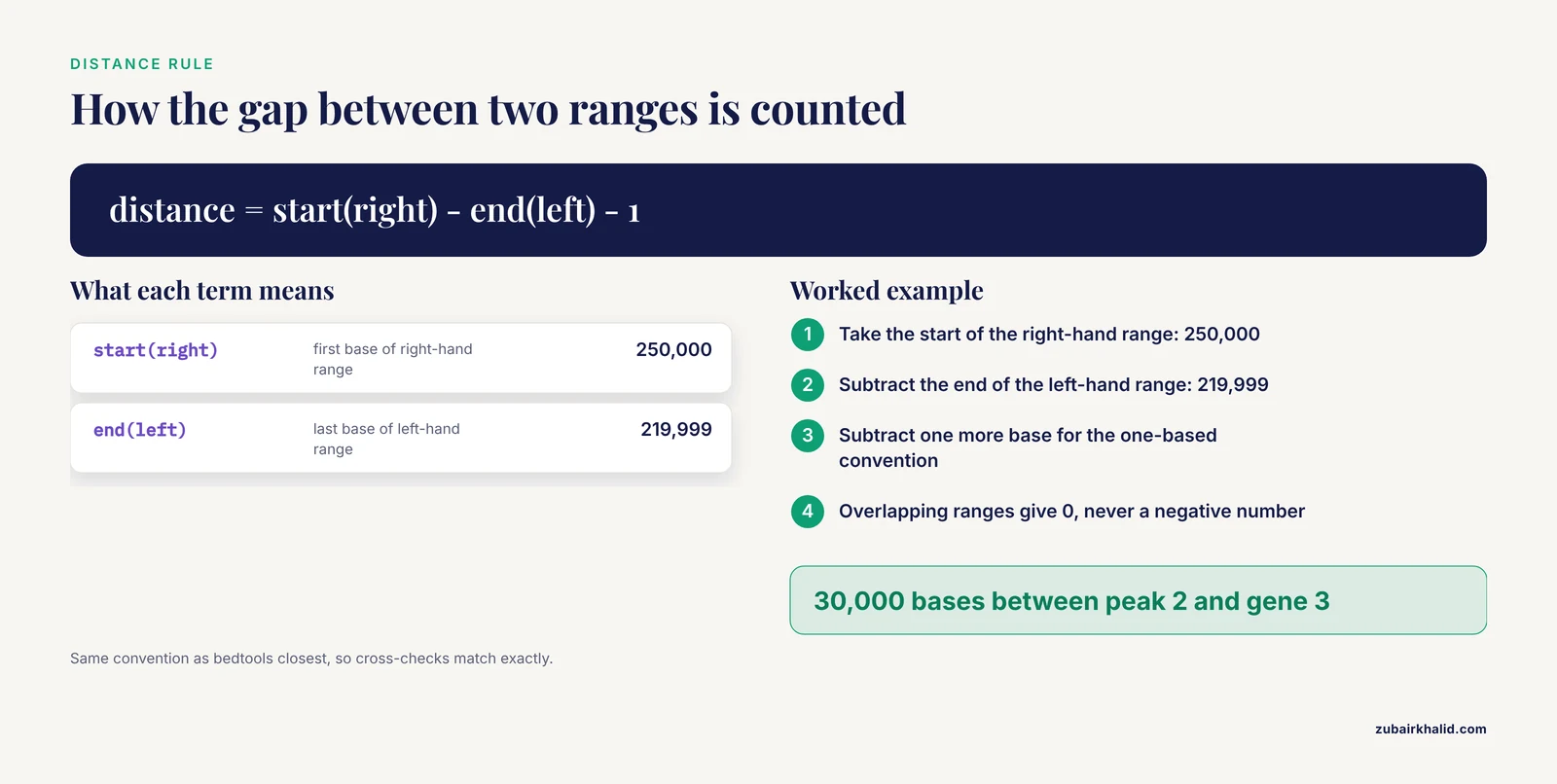
A neighbor is defined by distance, and the distance rule is worth memorizing because it drives every interpretation you will make: the distance between two non-overlapping ranges is the number of bases strictly between them. If range A ends at position 5,999 and range B starts at position 25,000, the distance is 25,000 minus 5,999 minus 1, which equals 30,000. If the ranges overlap at all, the distance is 0. Distances are never negative.

Before You Start: Installation and Setup

Install from Bioconductor using BiocManager. This is the standard installation path for any Bioconductor tutorial package.

if (!require("BiocManager", quietly = TRUE)) {
  install.packages("BiocManager")
}
BiocManager::install(c("GenomicRanges", "rtracklayer", "plyranges"))

Then load the core package:

library(GenomicRanges)

If you already have real data, load it directly into GRanges objects rather than through data frames. rtracklayer::import("peaks.bed") returns a GRanges object from a BED file, and rtracklayer::import("genes.gtf") does the same for GTF. The walkthrough below uses a small built-in example so you can check every number by hand.

Finding Nearest Neighbors with GenomicRanges in R, Step by Step

Step 1: Build the Query and Subject GRanges Objects

Create a subject of five genes on three chromosomes, with mixed strands, and a query of three peaks:

genes <- GRanges(
  seqnames = c("chr1", "chr1", "chr2", "chr2", "chr3"),
  ranges   = IRanges(start = c(1000, 50000, 200000, 800000, 500000),
                     width = c(5000, 10000, 20000, 15000, 30000)),
  strand   = c("+", "-", "+", "+", "-"),
  gene_id  = paste0("gene", 1:5)
)
genes

Expected output:

GRanges object with 5 ranges and 1 metadata column:
    seqnames          ranges strand |     gene_id
       <Rle>       <IRanges>  <Rle> | <character>
[1]     chr1     1000-  5999      + |       gene1
[5]     chr1    50000- 59999      - |       gene2
[2]     chr2   200000-219999      + |       gene3
[4]     chr2   800000-814999      + |       gene4
[3]     chr3   500000-529999      - |       gene5
-------
seqinfo: 3 sequences from an unspecified genome, no seqlengths

Now the query:

peaks <- GRanges(
  seqnames = c("chr1", "chr2", "chr3"),
  ranges   = IRanges(start = c(3000, 250000, 600000), width = 200),
  strand   = "*",
  peak_id  = paste0("peak", 1:3)
)

For real projects, replace this with rtracklayer::import() calls against your BED, GTF, or VCF files. The functions below behave identically regardless of where the ranges came from.

Step 2: Find the Single Nearest Feature with nearest()

nearest(peaks, genes, ignore.strand = TRUE)

Expected output:

[1] 1 3 5

This integer vector says that peak 1 is nearest to gene 1, peak 2 to gene 3, and peak 3 to gene 5. The indices point into the subject object, so you can retrieve full annotations directly:

nn <- nearest(peaks, genes, ignore.strand = TRUE)
genes[nn]$gene_id

Expected output:

[1] "gene1" "gene3" "gene5"

The most important parameter here is ignore.strand. Its default is FALSE, which means strand is considered and a query on one strand will never match a subject on the opposite strand. See Step 7 for a concrete demonstration of how that default produces a wrong answer. For peak-to-gene annotation, ignore.strand = TRUE is almost always what you want.

The select argument controls ties. With the default select = "arbitrary", when two subjects are exactly equally near, one is returned without a defined rule. With select = "all", nearest() returns a Hits object containing every tied neighbor.

When you omit the subject argument entirely, GenomicRanges searches for neighbors within x itself, and each range is not allowed to match itself:

nearest(genes)

Expected output:

[1]  2  1  4  3 NA

Gene 1 and gene 2 are each other's nearest neighbors on chr1 (a distance of 50,000 minus 5,999 minus 1, which is 44,000 bases), gene 3 and gene 4 are each other's nearest neighbors on chr2, and gene 5 has no other gene on chr3, so it gets NA. This pattern is the standard way to find, for example, the closest other peak in a peak set.

Step 3: Get Distances with distanceToNearest()

nearest() tells you which feature is closest. distanceToNearest() tells you that and how far, returning a Hits object:

hits <- distanceToNearest(peaks, genes, ignore.strand = TRUE)
hits

Expected output:

Hits object with 3 hits and 1 metadata column:
    queryHits subjectHits |   distance
    <integer>   <integer> |  <integer>
  [1]         1           1 |          0
  [5]         2           3 |      30000
  [2]         3           5 |      70000
-------
queryLength: 3 / subjectLength: 5

Check these numbers against the rule from the vocabulary section. Peak 1 spans 3,000 to 3,199 and gene 1 spans 1,000 to 5,999, so they overlap and the distance is 0. Peak 2 starts at 250,000 and gene 3 ends at 219,999, so the gap is 250,000 minus 219,999 minus 1, which is 30,000. Peak 3 starts at 600,000 and gene 5 ends at 529,999, so the gap is 70,000.

Extract the result as a plain data frame for downstream work:

as.data.frame(hits)
#   queryHits subjectHits distance
# 1         1           1        0
# 2         2           3    30000
# 3         3           5    70000

One behavior to know: distanceToNearest() returns all tied minimum-distance hits by default, so if two subject features are exactly the same distance from a query, that query produces two rows in the Hits object. The object can therefore have more rows than the query has ranges.

Step 4: Handle Overlapping Features Correctly

distanceToNearest() reports distance 0 for overlaps, but it still returns the nearest subject even when that subject overlaps the query. If you specifically want to exclude overlaps and find the nearest non-overlapping feature, combine precede() and follow(), which by construction never return overlapping ranges.

Step 5: Find Directional Neighbors with precede() and follow()

precede() returns, for each query, the subject index of the closest range that ends before the query starts. follow() returns the closest range that starts after the query ends. According to the GenomicRanges documentation, these functions treat all ranges as if they were on the plus strand, so "preceding" simply means at lower coordinates.

precede(peaks, genes)

Expected output:

[1] NA  3  5

follow(peaks, genes)

Expected output:

[1]  2  4 NA

Walk through peak 1 to understand the NA. Gene 1 spans 1,000 to 5,999, which overlaps the peak at 3,000 to 3,199. An overlapping range neither precedes nor follows the query, and no other chr1 range lies at lower coordinates, so precede() returns NA. Gene 2 lies to the right, so follow() returns index 2. Peak 3 sits to the right of gene 5, so precede() returns 5 and follow() returns NA.

If your actual question is "which gene is upstream of this peak, honoring gene strand," the cleanest approach is to reduce each gene to its transcription start site (TSS, the first base of the transcript) and search against those one-base ranges. This avoids all strand logic in the distance call:

tss <- c(
  resize(genes[strand(genes) == "+"], width = 1, fix = "start"),
  resize(genes[strand(genes) == "-"], width = 1, fix = "end")
)
hits_tss <- distanceToNearest(peaks, tss, ignore.strand = TRUE)
as.data.frame(hits_tss)

Expected output:

  queryHits subjectHits distance
1         1           3     1999
2         2           4    49999
3         3           5    70000

For peak 1 at 3,000 to 3,199, the nearest TSS is gene 1's TSS at position 1,000, giving a distance of 3,000 minus 1,000 minus 1, which is 1,999. Notice the answer differs from Step 3, where gene 1 was chosen because its body overlapped the peak. Asking a different question (distance to TSS versus distance to the gene body) legitimately changes the answer, which is why being explicit about the question matters.

Step 6: Annotate Peaks with the Nearest Gene, End to End

Here is the complete, copy-paste pattern you will reuse constantly in r for bioinformatics pipelines:

library(GenomicRanges)
library(rtracklayer)

peaks <- import("peaks.bed")            # query: GRanges from BED
genes <- import("genes.gtf")            # subject: GRanges from GTF/GFF

hits <- distanceToNearest(peaks, genes, ignore.strand = TRUE)

annotated <- peaks[queryHits(hits)]
annotated$nearest_gene <- genes[subjectHits(hits)]$gene_id
annotated$distance <- mcols(hits)$distance

head(as.data.frame(annotated))

Three details in this block prevent most real-world bugs. First, queryHits(hits) and subjectHits(hits) align every returned row, so the query and subject subsets stay in lockstep. Second, if distanceToNearest() returned multiple tied rows for some queries, peaks[queryHits(hits)] will contain duplicates for those queries, which is usually the behavior you want for tie-aware annotation. Third, mcols(hits)$distance pulls the distance column out of the Hits object.

Step 7: Understand the Strand Default with a Demonstration

This is the single most consequential default in the whole workflow. Consider a query on chr1 that lies between gene 1 (plus strand) and gene 2 (minus strand):

q <- GRanges("chr1", IRanges(34000, 34199), strand = "+")

nearest(q, genes)                       # default: ignore.strand = FALSE

Expected output:

[1] 1

nearest(q, genes, ignore.strand = TRUE)

Expected output:

[1] 2

The unstranded answer is gene 1 at a distance of 28,000, while the strand-blind answer is gene 2 at 15,800. Gene 2 is genuinely closer, but with the default setting it is invisible to the search because it sits on the opposite strand. For any annotation task where strand should not restrict the match, set ignore.strand = TRUE explicitly rather than trusting the default.

Step 8: Getting k Nearest Neighbors

GenomicRanges answers one-nearest-neighbor questions natively. For k nearest neighbors, the standard workaround is an iterative loop: find each nearest neighbor, remove it from the subject pool, and repeat. The following helper implements that idea:

k_nearest <- function(query, subject, k) {
  pool <- subject
  pool_id <- seq_along(subject)
  out <- NULL
  for (i in seq_len(k)) {
    if (length(pool) == 0) break
    h <- distanceToNearest(query, pool, ignore.strand = TRUE)
    round_result <- data.frame(
      query_id = queryHits(h),
      subject_id = pool_id[subjectHits(h)],
      distance = mcols(h)$distance,
      rank = i
    )
    out <- rbind(out, round_result)
    keep <- setdiff(seq_along(pool), subjectHits(h))
    pool <- pool[keep, ]
    pool_id <- pool_id[keep]
  }
  out
}

k_nearest(peaks, genes, k = 2)

Expected output:

  query_id subject_id distance rank
1        1          1        0    1
2        2          3    30000    1
3        3          5    70000    1
4        1          2    46800    2
5        2          4   549800    2

Read the output carefully because it teaches two lessons. Peak 3 has no second-nearest neighbor, because gene 5 is the only gene on chr3, so only one row exists for that query. And this algorithm removes each subject from the pool once it is claimed, so if one feature is the true nearest neighbor of many queries, those queries will pull different features at rank 2. For rigorous kNN statistics, such as the population-genetic genome scans that use k-nearest neighbor techniques over Fst and dxy values [2], use a purpose-built implementation rather than this annotation-grade workaround.

Step 9: A Tidy Alternative with plyranges

If you prefer pipes, plyranges wraps the same underlying machinery:

library(plyranges)
annotated <- peaks |>
  join_nearest_left(genes)

plyranges provides join_nearest_left, join_nearest_right, join_nearest_upstream, and join_nearest_downstream, which append the matched subject columns to the query. Under the hood these verbs rely on the same IRanges and GenomicRanges infrastructure that was built to support scalable range computation across Bioconductor [1], so results are consistent with the base functions shown above.

Key Functions and Arguments at a Glance

The distance formula to keep in mind for any two non-overlapping ranges A and B on the same chromosome: distance equals the start of the right-hand range minus the end of the left-hand range minus 1. Overlapping ranges give 0. This one-based, gap-counting convention matches what tools like bedtools closest report, which matters when you cross-check results.

How to Check That Your Results Are Right

Neighbor lookups feed directly into biological claims, so build verification into the workflow rather than treating it as optional.

First, construct a tiny example where you know the answer by hand, exactly as done in Steps 3 and 5. If the code cannot reproduce numbers you computed on paper, stop and debug before touching real data.

Second, cross-check a random sample against an independent tool. Export both sets as BED and run bedtools closest:

library(rtracklayer)
export(peaks, "peaks.bed", format = "bed")
export(genes, "genes.bed", format = "bed")

Then in a terminal:

bedtools closest -a peaks.bed -b genes.bed > crosscheck.txt

Compare a sample of, say, 50 rows against your R results. The distance conventions agree, so numbers should match exactly. Any discrepancy usually points to a strand or coordinate-style mismatch in one of the two pipelines.

Third, check global sanity signals in R:

sum(is.na(nn)) / length(nn)        # fraction of queries with no neighbor
summary(mcols(hits)$distance)      # distribution shape, spike at 0 means overlaps

A large NA fraction usually means a chromosome naming or strand problem rather than a biological finding. A suspicious spike at distance 0 usually means the query and subject sets share coordinates by construction, which may or may not be intended.

Fourth, spot-check a handful of high-stakes hits in a genome browser such as the UCSC Genome Browser or IGV. Five visual confirmations catch problems that no summary statistic will.

Common Mistakes and Limitations

• Trusting the strand default. As shown in Step 7, ignore.strand = FALSE silently hides opposite-strand candidates and can return a farther neighbor or NA. For annotation workflows, set ignore.strand = TRUE on every nearest, distanceToNearest, and distance call unless you have an explicit strand-specific reason not to.
• Expecting k neighbors from nearest(). The function returns exactly one neighbor per query under the default select = "arbitrary", and ties are broken without a defined rule. Use select = "all" to capture ties, and use the iterative approach from Step 8 for k greater than 1.
• Reading distance 0 as "zero bases apart." Distance 0 means the ranges overlap. If you need gap-like measures that exclude overlaps, use precede() and follow(), which never return overlapping ranges.
• Mismatched chromosome naming. If your query uses chr1 and your subject uses 1, the search fails with an error like the following:

  Error: 'levels(seqnames(x))' and 'levels(seqnames(subject))' must be the same

Fix it by harmonizing before the call, for example seqlevels(subject) <- seqlevels(peaks), or by using the GenomeInfoDb utilities such as keepStandardChromosomes() and seqlevelsStyle() to detect and convert naming styles. Assigning seqlevels that do not exist in the object produces a warning naming the unknown seqlevels, and that warning is a real bug signal, not noise.

• Mixing genome builds. If the query comes from hg19 and the subject from hg38, coordinates do not correspond and every distance is meaningless, even when the code runs without errors. Check seqinfo(peaks) and seqinfo(genes), confirm the genome identifiers agree, and lift over if they do not. Combining objects with incompatible seqinfo can also raise errors about genome information, which you resolve by harmonizing the seqinfo rather than suppressing the check.
• Indexing with NA results. genes[nn] where nn contains NA produces an NA range rather than an error, and the failure surfaces later as cryptic messages such as "subscript out of bounds" in downstream code. Filter matched pairs through a Hits object or drop NA indices explicitly before subsetting.
• Using nearest() for upstream and downstream questions. nearest() is direction-blind. precede() and follow() are the directional tools, and they apply plus-strand logic by design, so a gene on the minus strand has its biologically upstream end at higher coordinates. The 1-base TSS trick in Step 5 handles this correctly without manual strand bookkeeping.
• Assuming circular chromosome behavior. Neighbor searches do not wrap around chromosome ends unless the sequence is marked as circular in the seqinfo metadata. For mitochondria, plasmids, and other circular sequences, set the circular flag explicitly if wrap-around distances matter for your question.
• Performance anti-patterns. The neighbor machinery is efficient by design, using interval-based indexes that support scalable overlap and nearest neighbor detection across genome-sized data [1]. What destroys performance is an R-level loop calling nearest() once per query, or converting GRanges objects to data frames before the search. Call the vectorized function once on the full object and keep the data in GRanges form until the results are final.
• Interpreting a nearest-neighbor annotation as a statistical statement. Nearest feature assignment is an annotation, not evidence of regulation, enrichment, or association. Distance to the nearest gene says nothing about whether the peak interacts with that gene, and formal questions about enrichment or significance need a different analysis, such as permutation-based region testing.

Performance Notes for Large Datasets

For genome-scale queries, three habits keep things fast. Sort both objects by sequence and position with sort(). Keep seqlengths defined on both objects so the machinery does not have to make assumptions. And resist the urge to pre-filter with findOverlaps() and then run nearest() on the remainder, because nearest() already considers overlapping ranges as distance-0 candidates and handles them natively.

If you repeatedly annotate many query sets against one large subject set, keep the subject object as a single sorted GRanges variable and reuse it, rather than rebuilding it inside each function call. On modern hardware, single-shot neighbor searches against genome-wide gene annotations complete in seconds to minutes, and the underlying algorithms were designed and benchmarked for exactly this scale of operation [1].

Next Steps

Once nearest-neighbor annotation works, natural extensions include running the same queries against transcript databases built with GenomicFeatures, where transcript structures get first-class support within the same range infrastructure [1], wrapping the workflow into a reproducible script or package, and moving from nearest-neighbor annotation to formal enrichment testing with permutation-based methods. The plyranges verbs shown in Step 9 make it straightforward to fold neighbor annotation into longer pipe-based pipelines so that the whole analysis, from BED file to annotated table, lives in one reproducible script.

Frequently Asked Questions

Does nearest() in GenomicRanges consider strand?

By default it does, which surprises many users. With the default ignore.strand = FALSE, a query and a subject on opposite strands are never candidates, so you can get a farther neighbor or NA. For annotation work where strand should not restrict the match, set ignore.strand = TRUE.

What is the difference between nearest() and distanceToNearest()?

Both find the same single nearest feature. nearest() returns an integer vector of subject indices, while distanceToNearest() returns a Hits object that also carries the distance in its metadata column. Use distanceToNearest() whenever you need the distance as well as the identity of the neighbor.

Can GenomicRanges return the k nearest neighbors instead of just one?

There is no built-in k-nearest function. The standard workaround is an iterative loop that removes each matched subject between rounds, or findOverlaps() within a fixed window. Ties for the single nearest neighbor can be captured with select = "all".

Why do I get NA values from nearest()?

NA appears when no subject range qualifies for a query. The most common causes are a chromosome with no subject ranges, chromosome names that do not match between the two objects, and strand filtering that excludes every candidate.

How are ties handled when two subjects are equally near?

With the default select = "arbitrary", one of the tied neighbors is picked without a defined rule. Pass select = "all" to receive every tied neighbor as a Hits object, and note that distanceToNearest() includes all ties by default.

How do I find the nearest gene upstream or downstream of a peak?

Use precede() and follow(), which treat all ranges as if on the plus strand, or reduce each gene to a one-base TSS range with resize() and run distanceToNearest() with ignore.strand = TRUE so gene strand is honored correctly.

Is nearest() fast enough for millions of ranges?

Yes for typical genome-scale use, because the overlap and neighbor machinery is built on interval-based algorithms designed for scalable range computation. Avoid per-range R loops, sort your objects, and keep data in GRanges form rather than converting to data frames.

How can I check that my nearest-neighbor results are correct?

Verify a small hand-computed example first, cross-check a random sample of hits against bedtools closest or a genome browser, and monitor the NA rate and the distance distribution for anomalies such as an unexpected spike at zero.

Sources

1. Software for computing and annotating genomic ranges.
2. Genome scans for selection and introgression based on k-nearest neighbour techniques.
3. Neighbor GWAS: incorporating neighbor genotypic identity into genome-wide association studies of field herbivory.
4. Genomic copy number analysis of non-small cell lung cancer using array comparative genomic hybridization: implications of the phosphatidylinositol 3-kinase pathway.
5. Random forest imputation and genomic prediction for missing egg production time-series data in yellow-feathered broiler breeders.