Scaling Metagenomics Workflows in the Cloud
By Dr. Zubair Khalid, DVM, MS, PhD ·

By the end of this guide you will be able to take a metagenomics pipeline, profile it on a single sample, then fan it out across hundreds or thousands of samples on cloud infrastructure without wasting compute, money, or your weekend. You will learn how to stage data on object storage, configure an elastic compute backend, right-size memory and CPU requests, verify that scaled outputs match your pilot run, and audit cost and utilization after the fact.
To follow the walkthrough you need:
- A cloud account with permission to create compute environments and buckets. The commands below target AWS, which is the platform most metagenomics cloud infrastructure has been built and benchmarked on, so aws genomics tooling gets the closest treatment here.
- Nextflow (version 23.10 or later) installed locally or on a small submission host.
- Docker or Apptainer, so every tool runs in a container with pinned versions.
- A fastq directory with a handful of samples and roughly 10 GB of scratch space for the pilot.
- Familiarity with the command line. Nothing here assumes you administer a cluster.
The core idea of cloud bioinformatics is simple. Instead of buying hardware sized for your largest project, you rent capacity in exactly the shape and duration your workload needs, then release it. That utility model of computing, with near-unlimited capacity, burstable usage, and flexible payment, is what made large-scale genomics analysis practical in the first place [1]. Metagenomics stretches that model harder than almost any other sequencing application, because a single study can involve thousands of samples and because per-sample steps like assembly are memory hungry.
Why Metagenomics Belongs in the Cloud
The "bioinformatics bottleneck" was named over a decade ago, when researchers benchmarked common microbial genomics applications, including 16S rRNA analysis, whole-genome shotgun assembly and annotation, WGS metagenomics, and large-scale BLAST, on commercial cloud infrastructure using the CloVR virtual machine. They found considerable differences in computational requirements, runtimes, and cost across application types. While all 16S analyses completed on a single-CPU desktop in under three hours, microbial genome and metagenome assembly required substantially more compute [2]. That gap is the whole reason metagenomics cloud scaling exists as a discipline: cheap steps scale linearly, expensive steps do not.
The pressure has only grown. Sequence data now arrives faster than curated analysis can absorb it, and manual curation does not survive the scale-up to the million-microbial-genome era [3]. Public archives make the problem concrete. Before an NCBI Virus Discovery Hackathon, staff pre-assembled 141,676 metagenomic datasets from the Sequence Read Archive into contigs, and a subset of 2,953 datasets, roughly 55 million contigs, was then filtered to 4.2 million contigs of at least 1 kb for analysis. That exercise yielded direct insights into both the data and the cloud infrastructure needed to support efforts at that scale, including the analysis bottlenecks involved [4]. When your input is an entire archive rather than a single run, per-sample thinking breaks down and you need infrastructure that treats samples as a queue.
Production projects have since demonstrated what mature scaling looks like. The Celeste infrastructure, built for the All of Us sequencing program, processes fluctuating workloads of up to 9,000 whole-genome samples monthly. In 12 months of production within a single AWS Region, around 200 million serverless functions and over 20 million messages coordinated 1.8 million bioinformatics, quality control, and clinical reporting jobs, using serverless technology and container orchestration as the foundation [5]. Those numbers are from human WGS, not metagenomics, but the architectural lessons transfer directly: keep jobs small, keep orchestration stateless, and let the platform absorb workload swings.
What Scaling Actually Means for a Metagenomics Pipeline
There are three distinct scaling patterns, and confusing them is the root of most failed cloud runs.
Vertical scaling means giving one job a bigger machine. If a single metagenome assembly exhausts 256 GB of RAM, you request a 512 GB node. This works until the assembly needs more than the largest available instance, and you pay for the peak even when the job idles below it.
Horizontal scaling means running many jobs at once, each on a modest machine. Most of a metagenomics workflow is embarrassingly parallel across samples: quality control, host read removal, taxonomic profiling, and single-sample assembly can each run independently per sample. A 500-sample run is 500 independent jobs, limited only by how fast your compute environment can start containers.
Data-parallel scaling means splitting a single job's data across many machines. This matters when the reference resource, not the sample, is the bottleneck. Classic metagenomic profiling tools were designed against small representative genome collections and do not scale well to large ones, which motivated Flint, a profiler built on Apache Spark that maps reads against a 170 GB collection of 43,552 bacterial genomes on Amazon's Elastic MapReduce service, profiling 1 million paired-end reads against more than 40,000 genomes on 64 machines in 67 seconds [6]. Sparkhit took the same approach further, running 92 to 157 times faster than MetaSpark on metagenomic fragment recruitment and 18 to 32 times faster than Crossbow on preprocessing, analyzing 100 terabytes across four genomic projects on the cloud in 21 hours including cluster deployment and data download, and completing the entire Human Microbiome Project shotgun dataset in 2 hours [7].
A related trap deserves its own sentence. When a dataset grows by a factor of 10,000 or more, the performance-limiting factor can change entirely. A step that was I/O bound at 10 samples can become scheduler-bound at 10,000, and code that was fine on a workstation needs new paradigms in the cloud [1]. Benchmark at the scale you intend to run, not just at the scale you test.
Choosing a Workflow Engine and a Platform
Two decisions drive everything else: which workflow engine describes your pipeline, and where it executes.
For engines, Nextflow, Snakemake, and WDL/Cromwell dominate. The nf-core collection of community-maintained Nextflow pipelines, alongside tools like Bactopia, has become a standard way to assemble microbial and metagenomic analysis pipelines, and standardized pipeline frameworks now sit alongside the individual tools that became de facto standards, including FastQC, QIIME 2, Kraken2, SPAdes, GTDB-Tk, and Prokka [8]. For metagenomics specifically, nf-core/mag covers short- and long-read assembly, binning, and taxonomic profiling, and the Metagenomics-Toolkit provides a scalable, data-agnostic workflow that handles Illumina and Oxford Nanopore reads with quality control, assembly, binning, annotation, plasmid identification, dereplication, and genome-scale metabolic modeling, with optimizations for efficient cloud-based cluster execution [9].
For platforms, you have a spectrum from fully managed to fully self-built:
- Curated web platforms. NMDC EDGE provides a user-friendly, open-source web application for processing metagenome, metatranscriptome, and other microbiome data, built on three layers (web application, orchestration, and execution) that rely on software containers and accommodate both high-performance computing and cloud computing services [10]. Bio-Express similarly offers predefined metagenome pipelines alongside genome, transcriptome, and epigenome pipelines in a cost-effective cloud system [11]. These are the right entry point if you want standardized processing without managing infrastructure.
- Platform wrappers. AnVILWorkflow is an R package that executes workflows hosted on the AnVIL cloud platform directly from an R environment, simplifying cloud environment setup, input formatting, workflow submission, and result retrieval, with a metagenomics use case built on bioBakery [12]. It is well suited to exploratory analyses and bulk processing without direct infrastructure management.
- Portable workflow definitions. Publishing workflows in multiple formats (CWL, WDL, Nextflow) on registries such as Dockstore makes them runnable across platforms. rMATS-cloud demonstrated this portability by running the same workflow on Cavatica, Terra, and Seqera, and handling datasets with thousands of samples [13].
- Self-managed AWS. Nextflow or Cromwell driving EC2, AWS Batch, S3, and Spot instances gives maximum control. The rest of this walkthrough takes this route, because it teaches the mechanics that every other option hides.
Metagenomics Cloud Scaling Step by Step
This is the core walkthrough. It uses nf-core/mag on AWS Batch, but the sequence of steps applies to any engine and any pipeline, including the Metagenomics-Toolkit [9].
Step 1. Run the pipeline's test profile on one node
Before touching the cloud, prove the pipeline runs at all and that your container runtime works.
nextflow run nf-core/mag -profile test,docker -resumeThe test profile supplies tiny bundled data, so this finishes in minutes. Expected output:
N E X T F L O W  ~  version 24.04.2
Launching `nf-core/mag` [trusting_curie] DSL2 - revision: 2.4.0
...
[-] [ASSEMBLY (test_sample)] Process completed
Completed at 12-Nov-2026 09:14:07
Duration    : 41m 12s
Status      : SUCCESS
If this fails locally, it will fail in the cloud. Fix it here where iteration is cheap.
Step 2. Profile the per-sample resource envelope
Scaling decisions come from measurements, not guesses. Run one real sample and extract per-process resource use from the trace:
nextflow log -f name,status,peak_rss,duration,cpusExpected output looks like this:
name                      status   peak_rss   duration   cpus
NFCORE_MAG:MAG:FASTQC     CACHED   1.2 GB     3m 14s     2
NFCORE_MAG:MAG:HOST_REMOVAL  COMPLETED  28 GB  1h 12m   16
NFCORE_MAG:MAG:ASSEMBLY_MEGAHIT  COMPLETED  174 GB  3h 08m  24
Record the peak RSS (resident set size, the maximum memory the process actually touched) and duration for every process. In most metagenomics workflows, assembly and binning dominate memory, while read QC and profiling dominate job count. This single table drives every resource request you write later.
Step 3. Stage your data on object storage
Object storage (S3 in the AWS case) is the shared filesystem of cloud genomics. Every compute node pulls inputs from it and pushes outputs to it.
aws s3 sync ./fastq/ s3://my-metagenomics-bucket/raw/
aws s3 ls s3://my-metagenomics-bucket/raw/ | head
Expected output:
upload: ./fastq/sampleA_1.fastq.gz to s3://my-metagenomics-bucket/raw/sampleA_1.fastq.gz
upload: ./fastq/sampleA_2.fastq.gz to s3://my-metagenomics-bucket/raw/sampleA_2.fastq.gz
...
2026-11-11 08:02:11 1841009321 sampleA_1.fastq.gz
Verify the transfer by comparing object counts and sizes against the source directory. A mismatch here is invisible until step 9 and maddening to debug there.
Step 4. Build a samplesheet
Most community pipelines consume a CSV manifest. For short-read data in nf-core/mag:
sample,fastq_1,fastq_2
sampleA,s3://my-metagenomics-bucket/raw/sampleA_1.fastq.gz,s3://my-metagenomics-bucket/raw/sampleA_2.fastq.gz
sampleB,s3://my-metagenomics-bucket/raw/sampleB_1.fastq.gz,s3://my-metagenomics-bucket/raw/sampleB_2.fastq.gz
Upload it alongside the reads. Every row becomes one unit of horizontal scaling.
Step 5. Configure the AWS Batch executor
Create a Nextflow config that points work at S3 and execution at AWS Batch (a managed job queue that launches containers on EC2 as jobs arrive, and terminates them after):
workDir = 's3://my-metagenomics-bucket/work'

aws.region  = 'us-east-1'
aws.batch.cliPath = '/usr/local/bin/aws'

process {
  executor = 'awsbatch'
  queue    = 'my-metagenomics-queue'
  withLabel: 'process_high_memory' {
    memory   = 400.GB
    cpus     = 32
  }
}

docker.enabled = true
Each parameter matters:
workDiron S3 means the Nextflow work directory lives next to your data, so any node can resume any task.executor = 'awsbatch'makes Nextflow submit each process as a Batch job instead of running it locally.queuenames the Batch job queue attached to your compute environment. Create one compute environment on Spot capacity for stateless steps and one on On-Demand for anything you cannot afford to retry.withLabelblocks let you raise memory only for the processes that need it, using the labels the pipeline authors already defined. Setting 400 GB globally would multiply your bill by your worst process.
Set the compute environment's maximum vCPU count deliberately. That ceiling, not your ambition, is what limits fan-out.
Step 6. Launch the scaled run
nextflow run nf-core/mag \
  -r 2.4.0 \
  -profile aws_batch \
  -params-file params.json
with params.json:
{
  "input":  "s3://my-metagenomics-bucket/samplesheet.csv",
  "outdir": "s3://my-metagenomics-bucket/results"
}
The -r flag pins a pipeline release so a rerun next year resolves to identical code. Expected output:
N E X T F L O W  ~  version 24.04.2
Launching `nf-core/mag` [dizzy_lovelace] DSL2 - revision: 2.4.0
[-] [HOST_REMOVAL (sampleA)] Submitted process > 1 of 500
[-] [HOST_REMOVAL (sampleB)] Submitted process > 2 of 500
Within minutes the queue should show dozens of running jobs. If it shows one, your compute environment maximum vCPU setting is the bottleneck, not your pipeline.
Step 7. Monitor without babysitting
nextflow log -f name,status,duration | grep EXITED
aws s3 ls s3://my-metagenomics-bucket/results/ --recursive | wc -l
The AWS CLI flags after the bucket are standard argument syntax, so run the second command as written in your shell. Watch three signals: the fraction of tasks in a running state (a healthy fan-out is mostly running or succeeded), the Batch queue's oldest-job age (a growing age with an idle queue means a resource ceiling), and S3 result object growth.
Step 8. Diagnose the two failures you will actually get
The dominant failure at scale is the out-of-memory kill. Its signature is exit status 137:
Process `ASSEMBLY (sampleJ)` terminated for an incomplete execution
Command exit status:
  137
Exit 137 means the process was killed by SIGKILL, which on Batch is almost always the kernel out-of-memory handler after the task exceeded its container memory limit. Fix it by raising memory for that specific labeled process in your config, not globally, then rerun with -resume so completed tasks are not recomputed.
The second common failure is misconfigured storage:
An error occurred (NoSuchBucket) when calling the ListObjectsV2 operation:
The specified bucket does not exist
This is a typo in a bucket name, a wrong Region, or a work directory pointing at a deleted bucket. Check aws.region in your config and the bucket name in both workDir and your params file.
Step 9. Audit cost and utilization
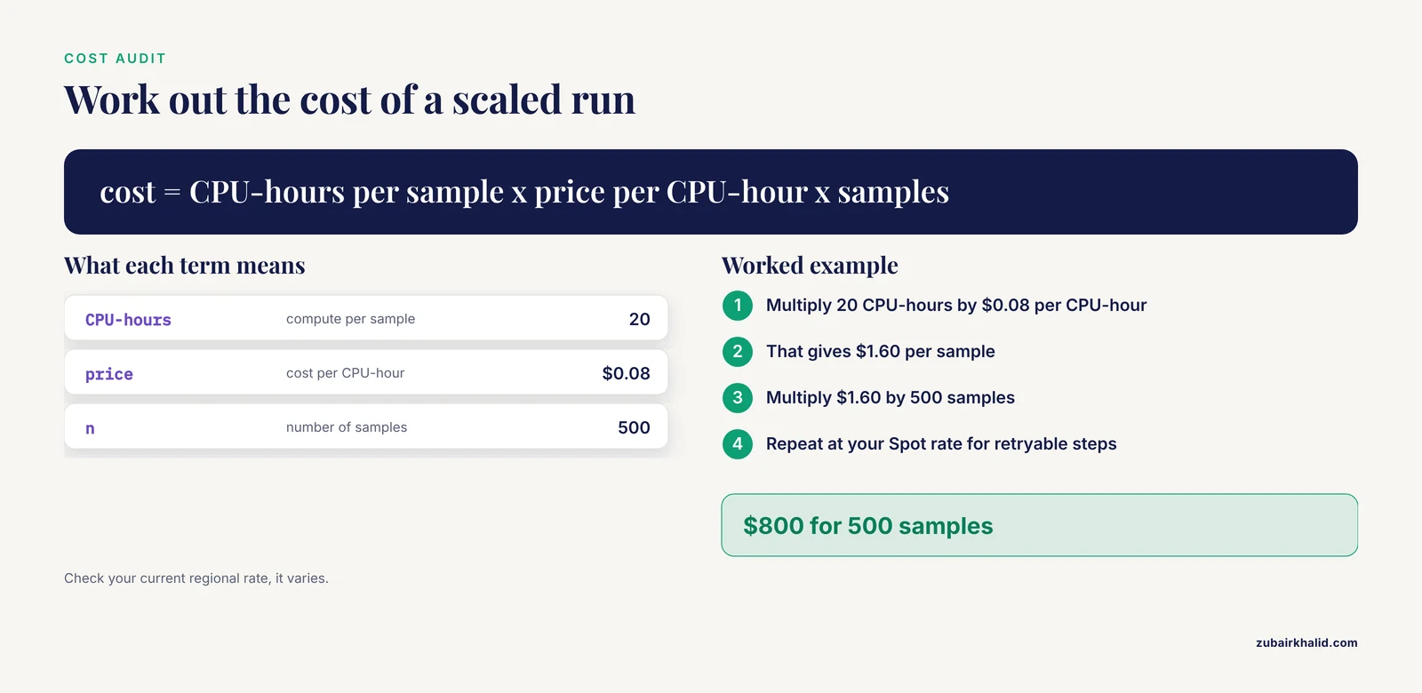
After the run, sum task durations from the trace and multiply by the CPU-hours you provisioned. The arithmetic is deliberately simple. If your profile showed an average of 20 CPU-hours of compute per sample and your instance class prices at 8 cents per CPU-hour (check your current regional rate, it varies), then:
cost per sample  = 20 CPU-hours x $0.08  = $1.60
cost for 500     = 500 x $1.60          = $800
Run the same calculation at your Spot rate, which is typically a large discount below On-Demand, and you have the business case for moving retryable steps to Spot. Compare the result against the benchmarking tradition established by the CloVR studies, which attached real dollar costs per analysis type on EC2 precisely so researchers could plan [2]. Keep the audit attached to this run only, and update it whenever your pipeline version or data profile changes.
Step 10. Prove scale before betting on it
Run 10 real samples end to end, then a 50-sample subset, then the full cohort. Compare per-sample outputs between the 10-sample pilot and the full run for a shared sample. If outputs drift, something in your configuration depends on run composition, and you want to find that at n=10, not n=500. The Metagenomics-Toolkit team validated their workflow at exactly this kind of scale, demonstrating capabilities on 757 sewage metagenome datasets [9], which is a reasonable order of magnitude for a first serious cloud campaign.
Scaling Patterns at a Glance
| Pattern | How it works | Best for | Real-world example |
|---|---|---|---|
| Per-sample scatter | One independent job per sample | QC, host removal, profiling, single-sample assembly | nf-core/mag on AWS Batch |
| Scatter-gather | Per-sample jobs, then a merge stage | Dereplication, cross-sample binning, co-occurrence analysis | Metagenomics-Toolkit dereplication stage [9] |
| Distributed data-parallel | One job's data split across many nodes | Profiling against very large reference collections, fragment recruitment | Flint on Amazon EMR [6], Sparkhit [7] |
| Serverless fan-out | Events trigger small, stateless compute units | Orchestration, file-level triggers, QC at extreme job counts | Celeste's serverless orchestration for All of Us [5] |
| Managed platform | Web application runs a curated, containerized workflow | Labs without dedicated engineers, standardized multi-omics processing | NMDC EDGE [10], AnVILWorkflow on AnVIL [12], Bio-Express [11] |
Metagenomics Cloud Scaling Tips
These tips are ordered by how much trouble they prevent.
- Profile before you provision. The single most valuable hour in metagenomics cloud scaling is the hour spent on step 2. Every memory number in your config should trace to a measured peak RSS.
- Right-size memory, and let the pipeline help. The Metagenomics-Toolkit includes a machine learning-optimized assembly step that adjusts peak RAM usage to match actual requirements, reducing the need for high-memory hardware [9]. Even without ML-driven sizing, matching requests to measured peaks cuts both cost and waste.
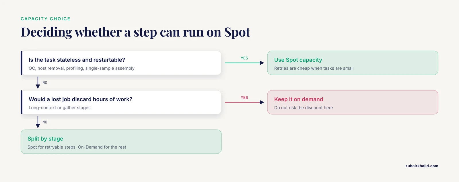
- Use Spot for everything that can retry. Per-sample assembly, QC, and profiling are stateless and restartable. Keep the On-Demand or equivalent fallback for the few stages where a lost job would discard hours of upstream work.
- Co-locate compute with data. Cloud performance-limiting factors shift as datasets grow [1], and one of the most reliable shifts is from compute-bound to data-movement-bound. Keep reads, references, and work directories in the same Region as the compute.
- Choose your Region with intent. Switching from an average data center to a more efficient one can reduce the carbon footprint of an analysis by approximately 34 percent, according to calculations with the Green Algorithms framework [14]. Region choice is a one-line config change with a real environmental effect.
- Know that faster is not always greener. Greater parallelization and faster processors reduce wall-clock time but can increase total carbon footprint, and memory over-allocation is itself a substantial contributor to an analysis's greenhouse gas emissions [14]. This is the strongest argument for measured resource requests rather than defensive over-provisioning.
- Containerize and pin everything. Containers are what make the orchestration and execution layers of platforms like NMDC EDGE flexible and portable between HPC and cloud [10]. Pin pipeline releases, container tags, and reference database versions together.
- Prefer cloud-native tools when references get big. If your profiling step struggles against a large genome collection, the fix is architectural. Spark-based tools demonstrated order-of-magnitude gains on large collections [6] and terabyte-scale preprocessing on the cloud [7].
How to Check That the Scaled Run Is Correct
Verification has three layers.
Per-sample identity. Pick three samples that ran in both your pilot and your full campaign. Their per-sample outputs (QC summaries, assembly statistics, profile counts) should match. Any drift means your configuration or input staging changed between runs.
Aggregate sanity. The nf-core-style pipelines emit a MultiQC summary across all samples, which lets you scan read counts retained at each filtering step, assembly sizes, and binning completeness across the entire cohort at once. Look for samples that are extreme outliers on any metric, since those are your staged-input or parameter mistakes.
Provenance. Keep the Nextflow trace, timeline, and report files in your results bucket. They record which container, which commit, and which resource limits produced every file. This is what turns "I ran it in the cloud once" into something a reviewer can reproduce, and reproducibility is one of the original promises that justified cloud platforms for large biological datasets [1].
Common Mistakes and Limitations
These are the errors that show up repeatedly in real cloud metagenomics campaigns.
- Scaling before profiling. Teams copy a colleague's config with 512 GB requests on every process, then wonder why 30 percent of a modest budget buys 10 percent of the samples. Defensive over-requesting also inflates carbon emissions through memory over-allocation [14].
- Treating the cloud as uniformly fast. A pipeline that ran fine on 10 samples can collapse at 10,000 because the bottleneck moved, as the computing-at-scale literature warns explicitly [1]. Re-benchmark at each order of magnitude.
- Ignoring fan-in stages. Scatter stages scale forever. Gather stages (dereplication, co-assembly, cross-sample binning) become single large jobs. The NCBI hackathon experience surfaced exactly these analysis bottlenecks and infrastructure gaps at scale [4]. Plan gather stages as their own, separately sized runs.
- Using tools that do not scale to modern references. Many standard profilers were built for small genome collections and degrade against large ones [6]. Check whether your tool was designed for your database size before assuming slow means misconfigured.
- Assuming one pipeline fits all data. Short-read Illumina and long-read Oxford Nanopore inputs need different handling, which is why workflows built to be data-agnostic across both exist [9]. Mixing read types in one samplesheet is a common silent failure.
- Unpinned versions and databases. A workflow without pinned releases, container digests, and frozen reference databases is not reproducible, only rerunnable. Standardized, containerized workflows exist precisely to prevent this [10].
- Believing cost is self-evident. Benchmarking work has shown considerable differences in cost across application types even for closely related analyses [2]. Your bill is a function of your resource requests, your instance pricing, and your retention choices, and you should audit all three after every campaign.
- Over-reading the outputs. Persistent challenges in microbial genomics include incomplete and biased reference databases [8], so a profile is an estimate conditioned on your database, not a census. Manual curation also does not scale to very large sample counts [3]. Individual biological claims still need expert review against the underlying data.
Frequently Asked Questions
What does scaling metagenomics workflows in the cloud actually mean?
It means running your per-sample analysis steps as many parallel jobs on rented compute, sized and paid for only while they run, rather than sequencing your samples through a single fixed server. The practical work is in choosing the right scaling pattern (scatter, scatter-gather, or data-parallel) and configuring the engine to exploit it.
How much compute does a metagenomics sample need?
It depends overwhelmingly on the assembly and binning steps, which is why the first step of any scaling effort is profiling one real sample and recording peak memory and duration per process. Light-read steps may need a few CPU-hours while assembly can need hundreds of gigabytes of RAM, and workflows that automatically adjust assembly memory to actual requirements reduce the need for high-memory hardware [9].
Is cloud bioinformatics cheaper than buying a server?
For bursty and large workloads, usually yes, because you pay only during the campaign. For small, steady workloads, a shared local server often wins. Benchmark studies have attached real dollar costs to common microbial genomics applications on cloud infrastructure precisely so this comparison can be made per analysis type [2], and your own per-sample cost calculation is the deciding number.
Which workflow engine should I use for metagenomics in the cloud?
Nextflow is the most common choice because of the nf-core ecosystem, which supplies production-quality metagenomics pipelines and standardized AWS profiles, and because tools like Bactopia sit in the same family [8]. WDL and CWL are equally valid and can make workflows portable across multiple platforms, as demonstrated by workflows published in all three formats [13].
How do I keep a cloud metagenomics pipeline reproducible?
Pin the pipeline release, container tags, and reference database versions, keep the work directory and results on object storage, and archive the trace and config files with the results. Platform-level efforts like NMDC EDGE build standardization and interoperability directly into their containerized orchestration and execution layers [10].
Can I run metagenomics pipelines on Spot instances?
Yes, for any stateless per-sample task with automatic retry, which in a typical metagenomics workflow is nearly everything. Keep non-retryable or long-context stages on standard capacity, and configure your engine to retry Spot interruptions automatically. The interruption risk is the price of the discount, and retries are cheap when tasks are small.
How do I scale to thousands of public SRA samples?
Treat the archive as a queue, not a download. Large community analyses have processed thousands of SRA metagenomic datasets through cloud pipelines in coordinated events, and those efforts revealed the real bottlenecks, such as assembly and data staging, that you will hit [4]. Stage data programmatically, keep per-sample jobs small, and let the queue absorb the scale.
How do I reduce the environmental footprint of cloud metagenomics?
Choose an efficient cloud Region, right-size memory instead of over-allocating, and upgrade to more efficient software versions where available. Quantification work with the Green Algorithms calculator found that switching to a more efficient data center can cut emissions by roughly 34 percent and that memory over-allocation is a substantial contributor to a tool's footprint [14].
Sources
- Computational biology in the cloud: methods and new insights from computing at scale.
- Resources and costs for microbial sequence analysis evaluated using virtual machines and cloud computing.
- Microbial bioinformatics 2020.
- NCBI's Virus Discovery Hackathon: Engaging Research Communities to Identify Cloud Infrastructure Requirements.
- Celeste: A cloud-based genomics infrastructure with variant-calling pipeline suited for population-scale sequencing projects.
- Large scale microbiome profiling in the cloud.
- Analyzing large scale genomic data on the cloud with Sparkhit.
- Advancements and challenges in bioinformatics tools for microbial genomics in the last decade: Toward the smart integration of bioinformatics tools, digital resources, and emerging technologies for the analysis of complex biological data.
- Metagenomics-Toolkit: the flexible and efficient cloud-based metagenomics workflow featuring machine learning-enabled resource allocation.
- Standardized and accessible multi-omics bioinformatics workflows through the NMDC EDGE resource.
- Bioinformatics services for analyzing massive genomic datasets.
- AnVILWorkflow: A runnable workflow package for Cloud-implemented bioinformatics analysis pipelines.
- rMATS-cloud: Large-scale Alternative Splicing Analysis in the Cloud.
- The Carbon Footprint of Bioinformatics.